- Regular article
- Open access
- Published:
Identifying and predicting social lifestyles in people’s trajectories by neural networks
EPJ Data Science volume 7, Article number: 45 (2018)
Abstract
In this research, we exploit repeated parts in daily trajectories in people’s movements, which we refer to as mobility patterns, to train models to identify and predict a person’s lifestyles. We use cellular data of a group (“society”) of people and represent a person’s daily trajectory using semantic labels (e.g., “home”, “work”, and “gym”) given to the main places of interest (POI) he has visited during the day, as determined collectively based on interviewing all people of the group. First, in an unsupervised manner using a neural network (NN), we embed POI-based daily trajectories that always appear together with others in consecutive weeks and identify the result of this embedding with social lifestyles. Second, using these lifestyles as labels for lifestyle prediction, user POI-based daily trajectories are used to train a convolutional NN to extract mobility patterns in the trajectories and a dynamic NN with flexible memory to assemble these patterns to predict a lifestyle for a trajectory never-seen-before. The two-stage algorithm shows model accuracy and generalizability in lifestyle identification and prediction (both for a novel trajectory and a novel user) that are superior to those shown by state-of-the-art algorithms. The code for the algorithm and data sets used in our experiments are available online .
1 Introduction
Thanks to the increasing use of GPS devices, wearable sensors, and location-based services, a significant amount of data on human movement has been collected. This data can be used for analyzing the mobility patterns of people, their behavior, and lifestyles. For example, in a recent study [1], we extended latent Dirichlet allocation (LDA) to capture the temporal relations in mobility patterns that are reflected in a specific person’s trajectories of movement, in order to identify his lifestyle. In this study, we extend the previous study to identify lifestyles from trajectories for a society of people, and not only for a specific person, as people share different aspects in their behavior and lifestyles, and shared information that is exploited from mobility patterns for an individual may enhance our understanding and prediction capability of the behavior and lifestyle of another individual, and imply on those for the society itself. Identifying lifestyles for a single person is vital in a wide variety of fields, such as in psychiatry, where a doctor or caregiver can monitor the state of a specific patient, say having bipolar disorder, in order to intervene in situations such as in mania or depression periods, that pose a danger to the patient or others. Identifying lifestyles for groups of people may help in distinguishing these groups, e.g., patients with bipolar disorder having different characteristics, tourists among locals in a specific city, or people with various special needs.
In this study, we are interested in identifying and predicting social lifestyles in people’s trajectories of movement. For the identification part, we suggest learning user lifestyles by capturing temporal relations between trajectories using embedding. We do this by extending word embedding—traditionally implemented within the word2vec [2] framework using a neural network (NN)—to trajectory embedding by associating a word in a sentence with a mobility trajectory made by a user during a two-week period. After modifying the raw data of a user’s locations, which consist of latitude, longitude, and timestamps, into “sentences” (in the context of word embedding) of two consecutive weeks, we apply trajectory embedding by the word2vec algorithm to cell-phone user data, and demonstrate the advantage of this embedding in capturing dependencies between trajectories. Using t-distributed stochastic neighbor embedding (t-SNE) [3]—a non-linear dimensionality reduction algorithm—we cluster these embedded trajectories to identify human lifestyles.
For the second task of predicting lifestyles for a new mobility pattern (of a known or an unknown user) based on already identified lifestyles, we assume that:
-
Trajectories reflecting the same lifestyle do not have to be identical or very similar, but they should share specific sub-sequences with common semantic meaning;
-
The order (sequence) of places of interest (POIs; most frequently visited places) along a trajectory, as well as past and future POIs on the trajectory, indicate on the lifestyle they represent; and
-
Correlation between POIs along a trajectory (measured, e.g., by the POIs’ co-occurrence) imply on the lifestyle reflected by this trajectory.
Prediction of a lifestyle for a trajectory can be related to text classification [4], where we associate a person’s POIs, trajectories, and lifestyle with words, text, and text classification, respectively. However, in traditional text classification, feature engineering is conventionally needed, and the order of the words is assumed to be unimportant (the “bag of words” assumption). To avoid feature engineering, we can apply end-to-end NN solutions [5], and to dispense with the “bag of words” assumption, we can utilize, e.g., n-grams or hidden Markov models (HMMs) [6]. In this study, we extend elements of sequence text classification [5] to the prediction of a lifestyle (a latent unknown variable) from human mobility patterns that are extracted from trajectories of movement.
Therefore, our approach for identifying and predicting social lifestyles in people’s trajectories is based on four pillars, in which the first two are a pre-processing stage, and the last two are the identification and prediction stages:
-
Embedding of POI-based daily trajectories that always appear together with others in consecutive weeks in lifestyles using word2vec [7] and t-SNE [3] from cellular data of a society of people, and not of only a single person [1]. This embedding provides lifestyle (abstract) labels to trajectories in an unsupervised manner, which are then used to train supervised system elements of the other pillars;
-
Embedding of POIs in lifestyles using an NN in order to project semantic (categorical) POIs, e.g., “home”, “work”, “gym” (as collectively determined by the society) to a continuous representation that suits system elements for social lifestyle prediction, while keeping semantically close POIs (with respect to lifestyles) also close in their embedding;
-
Identifying high-frequency sub-sequences of co-occurring POIs (i.e., mobility patterns) that are associated with the lifestyles embedded by the first pillar using a convolutional neural network (CNN) (similarly to identification of edges and other features that compose image objects, which is the most prevalent task of CNN); and
-
Predicting a lifestyle based on a never-seen-before mobility pattern in a trajectory of known or novel users using long short-term memory (LSTM) of flexible memory, which is a variation of the recurrent NN, and bidirectional LSTM (BLSTM), which also allows future sub-sequences besides past ones in the trajectory to contribute to the prediction.
Our contribution is in developing methods for unsupervised inference of latent lifestyles and lifestyle identification and prediction, and generalization of these capabilities for a society of people to identify and predict social lifestyles for novel mobility patterns never-seen-before.
In Sect. 2, we survey the relevant literature to our study. In Sects. 3 and 4, we respectively describe our methodologies for identifying and predicting a lifestyle by a trajectory. In Sect. 5, we demonstrate the ability of our method in two scenarios: one of predicting a lifestyle for a novel sequence and the second of predicting a lifestyle for a novel user. In Sect. 6, we summarize our contribution. Finally, in Sects. 7 and 8, we respectively conclude and suggest avenues of new research.
2 Related work
Learning a user’s mobility pattern is challenging because it involves many aspects in the user’s life and levels of knowledge, combined with a high level of uncertainty. This challenge is historically connected to systems optimization, e.g., in predicting the density of cellular users to perform resource reservation and handoff prioritization in cellular networks [8]. As information collected from cellphones has become increasingly personal, models have become more user-specific. Thus, predicting a mobility pattern is at a higher level of learning than finding the geographic coordinates of locations, enabling prediction of significant places for individuals [9].
Most research in learning mobility patterns today stems from the large amount of information currently collected on users from different sources, information that in our case can help predict human behaviors and lifestyles. Such information has been based, e.g., on accelerometers [10], state-change sensors [11], or a system of RFIDs [12]. In a series of studies, [13, 14] presented the prediction and correlation of human activities based on information from the user’s location. [15] proposed the use of eigenbehaviors to predict human behavior. Eigenbehaviors describe the important features of observed human behavior in a specific time interval, which may be related to lifestyles, and allow direct comparison between movement patterns of different people. The authors described behavior that changes over time, and showed how eigenbehaviors build behavior structures.
Discovery of mobility patterns and prediction of users’ destination locations, both in terms of geographic coordinates and semantic meaning, was demonstrated [16] without using any semantic data voluntarily provided by a user or sharing of data among the users. The proposed algorithm allows a trade-off between prediction accuracy and information and shows that the predictability of user mobility is strongly related with the number and density of the users’ locations, as learned from the data of each user.
A recent review [17] surveyed and assessed different approaches and models that analyze and learn human mobility patterns using mainly machine learning methods. The authors categorized these approaches and models in a taxonomy based on the positioning characteristics, scale of analysis, properties of the modeling approach, and class of applications they can serve. They found that these applications can be categorized into three classes: user modeling, place modeling, and trajectory modeling, each class with its own characteristics.
Also LDA [18] can be applied to identify human lifestyles from mobility patterns, but since it makes the assumptions of “bag-of-words” and the order of documents, in order to capture temporal relations in the mobility patterns, we needed in a previous study to relax these assumptions by extending the LDA [1]. In contrast, word2vec is a less complex model that eliminates the need to consider any assumptions.
Following its introduction [2], word2vec has generally been applied in natural language processing [19, 20]. Because of the efficacy of this model’s framework in capturing the correlations between items, it is employed in network embedding [21], user modeling [22], item modeling [23], and item recommendation [24, 25].
There is recent work on word embedding also in the context of POIs. For example, [26] suggested how to find these POIs. [27] showed how to use word2vec in order to create POI vectors to perform better POI recommendations for users. They treat a user as a “document,” check-in sequence as a “sentence,” and each POI as a “word.” The difference in our work is that we used word2vec for sequence (i.e., trajectory) embedding and not POI embedding, similar to paragraph2vector [28] and other word2vec variants [29, 30] proposed to enhance the word2vec framework for specific purposes. Gao et al. [31] performed trajectory embedding as a post-processing stage in their mobility patten analysis, but not for lifestyle prediction.
3 Identifying a lifestyle by trajectory
In this section, we identify the lifestyle by embedding according to following stages:
-
1.
Finding significant POIs ⊳ Sect. 3.2
-
2.
Finding semantic meaning for POIs ⊳ Sect. 3.3
-
3.
Creating a semantic trajectory ⊳ Sect. 3.4
-
4.
Clustering unique semantic trajectories ⊳ Sect. 3.5
-
5.
Building a trajectory representation of two consecutive weeks ⊳ Sect. 3.6
-
6.
Embedding of trajectories using Trajectory2vec ⊳ Sect. 3.7
-
7.
Identifying a lifestyle for a trajectory ⊳ Sect. 3.8
After raw data of longitude, latitude, and timestamps have been collected from users using the Google Location History app [32] (Sect. 3.1), preprocessing is performed in five stages. The first stage of preprocessing is finding significant POIs, and the second is giving them semantic meaning. The third stage is creating semantic trajectories of POIs, and the fourth is clustering trajectories to unique semantic trajectories. Preprocessing is completed by building a trajectory representation of two consecutive weeks. Then identification of lifestyles by embedding is performed in two stages (Stages 6 and 7). Figure 1 shows the preprocessing stages from finding significant POIs to clustering unique semantic trajectories, and Fig. 2 demonstrates the process of trajectory embedding with word2vec and t-SNE.

Preprocessing. The preprocessing stage from raw data to clustered trajectories. d is the cell size; A, B, C, D, and O are POIs (O is a POI outside the map); g is the number of trajectories (and days); gT is the number of unique trajectories, where each day is represented by a 24-hour trajectory; and N is the number of trajectory clusters

Identifying a lifestyle. The process for identifying a lifestyle to trajectory. N (3000) is the trajectory clusters number, n is the number of the hidden layer in the word2vec model, and LS is the lifestyle number
3.1 Collecting data
The Google Location History app records the coordinates and timestamps of locations collected from Android users. An Android user can download these records in a JSON file. This file includes the longitude and latitude of the location, the timestamp, and more metadata about the accuracy of the recorded location, the speed of the user at the time of the record, and type of movement, e.g., walking, biking, riding in a vehicle, etc., at the time of the record. In this research, we chose to consider only the longitude and latitude of the locations and their timestamps.
With their permission, we collected the data from 38 users, who agreed to assign semantic meanings, e.g., home, work, etc., to their POIs.
In the next section, we decribe how we changed the Google Location History into POIs.
3.2 Finding significant POIs
We used two-week time periods to capture the previous week’s influence on the current week. Because the Google Location History may have missing data, e.g., periods of time with no records, we selected only two-week periods which had no more than 24 hours of missing data in each week.
The recorded latitude and longitude are not always precise because of the frequent use of cellular networks rather than GPS for recording the Android user’s choice. Because there are places with low coverage of cellular towers, the recorded location may not be as accurate. Due to low accuracy, different close places may be recorded as having the same semantic meaning, adding noise to the raw data. Thus, we grouped nearby places to reduce noise in the identification of the user’s most significant places. By converting the geographic map into a grid with a cell size of (approximately) \(10\times 10\ \mbox{m}^{2}\) (size d in Fig. 1) and rounding the latitude and longitude according to: \(\mathrm{new}_{x} = \mathrm{round}(\mathrm{old}_{x} * 10,000 / 5) * (5/10,000)\) (10,000 and 5 are parameters to create the grid cell size), we defined every grid cell as a POI, and every longitude and latitude point was related to a POI by its geographical position (See Fig. 1).
To select the above values—the 24-hour time window and \(10\times10~\)m grid size—we needed to check ranges of values that reasonably manifest a typical human lifestyle and places of visit. We checked time-window sizes between six and 48 hours with a six-hour jump because these periods are significant in a person’s life, and grid-cell sizes between two and fourteen meters with a two-meter jump because these sizes are typical to rooms, shops, offices, etc. that establish places people visit/stay. Besides their plausibility, the two selected values achieved the highest accuracy in lifestyle classification by a naive Bayesian classifier (NBC) following a simple preprocessing stage we applied to the data. However, for this preprocessing stage, we needed results that were derived only at later stages, providing feedback to this earlier stage. First, we established a vocabulary of 34 POIs having semantic meanings to our “society” of 38 people (see Sect. 3.3). Second, we created n-grams of semantic sub-sequences of n POIs in the trajectories. We used an n-gram of size three because this size is half of the smallest time-window size of six, which represents a meaningful unit in a person’s life. For example, if we had a trajectory of six POIs: \(\{\mathrm{home}, \mathrm{school}, \mathrm{work}, \mathrm{work}, \mathrm{gym},\text{ and }\mathrm{home}\}\), the 3-grams extracted were: \(\{\mathrm{home}, \mathrm{school}, \mathrm{work}\}\), \(\{\mathrm{school}, \mathrm{work}, \mathrm{work}\}\), \(\{\mathrm{work}, \mathrm{work}, \mathrm{gym}\}\), and \(\{\mathrm{work}, \mathrm{gym}, \mathrm{home}\}\). Each of the L unique 3-grams (\(L=4\) in this example) establishes a “term” for which, in the third stage, we computed frequencies over all terms. Fourth, we represented each trajectory as an L-dimensional vector for which its ith element is the term frequency (TF) of the ith term identified in this trajectory. Finally, we trained the NBC using this trajectory representation, while corresponding lifestyle classes were derived following trajectory embedding and identification, as will be described in Sect. 3.7 and Sect. 3.8, respectively. Evaluating the classification accuracy of NBCs trained using different combinations of time windows and grid sizes using the validation set, we could identify the most appropriate values, as described above.
Finally, we filtered non-significant POIs, i.e., places a user visits infrequently, and kept only the most frequent POI in each hour. We counted the appearances of these POIs, and if a POI was not in the 10% that most frequently appeared, it was considered “rare” and was labeled Other (The Other label appeared on average 12.34% out of 24 hours on the trajectories of each user). Non-rare POIs are the building blocks of the trajectories, which are constructed from the POIs and the timestamp.
In the next section, we describe how we found the semantic meaning of the POIs for a specific user.
3.3 Finding semantic meaning for POIs
After finding the POIs of each of the 38 users, we created a custom map (with Google My Maps of [32]) for every user with his POIs. This map was shared with the user, who gave every POI semantic meaning according to Table 1, which was created based on the semantic meanings of all POIs of all users. Sharing the semantic meanings of POIs among users enabled the establishment of a common vocabulary of semantic POIs (Table 1) for all users. Then we created for every user a hash table for his POIs, i.e., a semantic meaning for each of his POIs.
In the next section, we describe how to build the trajectories from the POIs for each user.
3.4 Creating a semantic trajectory
We limited a trajectory, i.e., places a user visited sequentially in a given interval of time, to the length of a day, a significant time period in a user’s life. Thus, to form a trajectory, we created a vector with 24 slots, each representing one hour (Fig. 1). Each slot was assigned a number that represented the semantic meaning (Table 1) of the most frequent POI at this specific hour on this specific day. Thus, the daily trajectory was defined as a string of 24 letters (POIs). If there was no record at a specific hour, this hour was assigned the semantic value of No Record.
In the next section, we describe how we reduced the trajectory dimension.
3.5 Clustering unique semantic trajectories
The number of possible trajectories is 3424, for which 34 is the number of possible POIs (see Table 1) and 24 is the number of slots in the trajectories. Although the actual number of trajectories is usually close to the number of days in this dataset, if we want to employ word2vec methods, we need to further reduce this number to create a strong co-occurrence between the trajectories. Therefore, we performed unsupervised learning with a hierarchical clustering algorithm and the edit distance metric on the unique trajectories to achieve a more compact trajectory representation (Fig. 1). The edit distance measures the similarity between two temporal sequences of equal length. We chose this distance because the sequences must be the same length. The number of clusters was determined empirically to be a quarter of the number of unique trajectories of all the users, e.g., if the number of unique trajectories of all the users was approximately 12K, so the number of clusters was determined to be 3K (gT in Fig. 1). Labels in \(\{1,N\}\) for all clusters are kept using a hash table.
In the next section, we describe how we built weekly-time dependances between the trajectories.
3.6 Building a trajectory representation of two consecutive weeks
Since we try to show that the previous week and trajectory impact on the current trajectory, we input here into our model two consecutive weeks to validate this impact. That is, a series of seven consecutive trajectories (days) was grouped in a week, beginning on a Sunday and ending on a Saturday, and two-consecutive weeks were grouped together to make a 14-dimensional sample (observation). Similarly, each other couple of consecutive weeks in the user’s database were grouped to form another sample, and all these samples formed the data set for this user.
In the next section, we describe how we embedded the different trajectories to continuous vectors.
3.7 Embedding of trajectories using Trajectory2vec
Word2vec is an NN embedding model from natural language processing (NLP), which is able to embed words into word vectors [2]. The model was extended to different research areas, other than NLP, such as an extension of word vectors for n-grams in biological sequences (e.g., DNA, RNA, and proteins) for bioinformatics applications, as proposed by Asgari and Mofrad [33]. Also, another extension of word vectors for creating a compact vector representation of unstructured radiology reports has been suggested by Banerjee et al. [34].
In this work, we establish a connection between word embedding and what we call “trajectory embedding”. If the POIs’ sequence in the trajectory can be considered as letters, so the trajectories can be considered as words, and a two-week period is our text. Therefore, a word2vec model can be used to embed trajectories, each is a sequence of 24 consecutive POIs, in trajectory vectors, which are 14-dimensional representations of two consecutive weeks (Sect. 3.6).
In neural language models, such as word2vec, the word probability given other (previous and next) words is:
where \(v^{\prime}_{w_{t}}\) is the output vector for input word \(w_{t}\) [this is column t in weight matrix \(\textbf{W}^{\prime}\) (Fig. 3)], V is the size of the vocabulary, m is the number of previous and next words to look at, and h is equal to \(W^{T}x\), e.g., the hidden vector of the input layer. In Fig. 3, the input and output layers indicated as x and v, respectively, are one-hot vectors to each word w in the data. Word2vec is a word embedding algorithm based on an NN, and it can have different architectures. Although it has several implementations, we limit our discussion to only CBOW.

Word2vec. Word2vec represented as an NN
Continuous bag-of-words (CBOW). In CBOW (Fig. 4), word \(w_{t}\) is predicted according to its context, i.e., the words surrounding it (the context words) where their order has no impact. \(w_{t}\) in (Eq. 1) is the output, and the context window of size 2m, \(w_{t \pm m}\) is the input (C in Fig. 4 is equal to 2m).

CBOW. CBOW model (See [7])
Negative sampling (NEG). Sampling-based approaches do away with the softmax layer. They do this by approximating the normalization in the denominator of the softmax (Eq. 1) with some other loss that is inexpensive to compute. However, sampling-based approaches are only useful at training time, while during inference time, the full softmax still needs to be computed to obtain a probability.
NEG is an alternative to hierarchical softmax [2], which is an approximation to noise contrastive estimation (NCE) [35]. NCE can be shown to approximate the loss of the softmax as the number of samples k increases. NEG simplifies NCE, and does away with this guarantee, as the objective of NEG is to learn high-quality word representations rather than achieving low perplexity on a test set, as is the goal in language modeling.
NEG also uses a logistic loss function to minimize the negative log-likelihood of words in the training set. For every word \(w_{t}\) given its context \(c_{t}\) of m previous words \(w_{t-1},\ldots,w_{t-m+1}\) in the training set, we generate k noise samples \(\tilde{w}_{tk}\) from a noise distribution Q (in NEG, we set the most expensive term, \(kQ(w)\), to 1). We can sample from the uni-gram distribution of the training set. As we need labels to perform our binary classification task, we designate all correct words \(w_{t}\) given their context \(c_{t}\) as true \((y=1)\) and all noise samples \(\tilde{w}_{tk}\) as false \((y=0)\). NEG calculates the probability that a word w comes from the empirical training distribution P given a context c as follows:
\(P(y=1|w,c)\) can be transformed into the sigmoid function:
And then the logistic regression loss is:
While NEG may thus be useful for learning word embeddings, its lack of asymptotic consistency guarantees makes it inappropriate for language modeling.
Each element of the 14-dimensional trajectory representation of two consecutive weeks (Sect. 3.6) (which represents a day) holds the index of the cluster (Fig. 2), of the 3K possible clusters (Sect. 3.5), to which the corresponding trajectory was clustered. Then if, for example, we choose to train the CBOW model, each of the 14 trajectory representations is turned using 1-of-c coding to a 3000-dimensional vector, where all vector elements are zero except that corresponding to the cluster index, which is one. Such a vector for a predicted trajectory (day) feeds the NN output layer, while similar vectors for the context window, i.e., trajectories for the previous and following days, feed the NN input (Fig. 4). That is, we use neighboring days to predict the current day using the CBOW model. At the end of the learning process, the (\(3000 \times n\)) input-hidden and (\(n \times 3000\)) hidden-output weight matrices are seen as embedded trajectories (n is the dimension of the trajectory vector; Fig. 4), whose dimensions are further reduced (Sect. 3.8) using t-SNE from n to two (Fig. 2) before being clustered and identified by a lifestyle.
In the next section, we describe how we found the lifestyles from the embedded trajectories.
3.8 Identifying a lifestyle for a trajectory
After trajectory embedding (Sect. 3.7), we reduced the dimension of the embedded trajectories (represented by the two NN weight matrices) using non-liner dimensionality reduction by t-SNE (Fig. 2). The t-SNE [3] algorithm is well suited for embedding high-dimensional data into a two-dimensional space in such a way that similar objects (trajectories in our case) in the high dimension are projected close to each other in the two-dimensional space, and dissimilar objects are projected far apart.
The t-SNE algorithm has been used in a wide range of applications including cancer research [36], music analysis [37], and bioinformatics [38]. The algorithm has two main stages. First, a t-SNE builds a probability distribution over all pairs of objects in the high-dimensional map. The objects have a very high probability to peak if they are similar, and very low probability to peak if they are dissimilar. Second, the t-SNE defines a similar probability distribution over all pairs in the low-dimensional map, and it tries to minimize the KL-divergence between the two distributions concerning the locations of the points on the map.
By clustering hierarchically these two-dimensional trajectory clusters with the Euclidean distance, we can associate each trajectory cluster with a lifestyle (Fig. 2). Note that hierarchical clustering groups the N two-dimensional original clusters into a reduced number of hierarchically-clustered clusters, each identified with a lifestyle, and this lifestyle is associated with all the original clusters grouped in the hierarchically-clustered clusters.
4 Predicting a lifestyle by trajectory
In this section, we show an approach to predict a lifestyle by a trajectory with a system of NNs. Based on the trajectories identified in an unsupervised manner for each user individually (Sect. 3), we can now use all unique trajectories of all the users to train this NN system to predict a lifestyle for a trajectory in a supervised manner.
4.1 Predicting a lifestyle by trajectory with NN
In predicting lifestyles, there is a high level of uncertainty even when trying to predict the lifestyles of individual people. This uncertainty increases when we predict the lifestyles of a society of people. To lower the uncertainty and to be able to accurately predict lifestyles, we exploit:
-
1.
Semantic similarities along trajectories representing the same lifestyle;
-
2.
Sub-sequences of co-occurring POIs that compose mobility patterns in the trajectory; and
-
3.
The order of the POIs in the trajectory, and temporal relations between past/future POIs and the current one.
To accomplish these three features, our system of three NNs: (1) Embeds POIs in lifestyles accompanied by t-SNE to project categorical POIs, e.g., “home”, “work”, “gym” onto a continuous representation (needed by the next NN, which is CNN), while keeping semantically close POIs (with respect to lifestyles) also close in their embedding (Sect. 3.7); (2) Detects high-frequency sub-sequences (mobility patterns) of size n of co-occurring POIs that are associated with the lifestyles using a CNN with a filter size of n (Sect. 4.1.3); and (3) Exploits the order of the POI sequences in the trajectories to classify a trajectory to a lifestyle using a flexible memory to the past by the LSTM (Sect. 4.1.1) or using a flexible memory also to the future (as we have the whole trajectory) by the BLSTM (Sect. 4.1.2), which can potentially improve prediction by considering temporal relations from the past and to the future for each POI in the sequence.
Therefore, we explore five NN system architectures based on different intuitions and combinations of these features, each implemented as an NN layer, and compare these architectures (all explained below) to the recurrent neural network (RNN) as a reference:
-
RNN: Word embedding layer → Dropout → RNN layer → Dropout.
-
LSTM: Word embedding layer → Dropout → LSTM layer (Fig. 5) → Dropout (see Fig. 6).
Figure 5 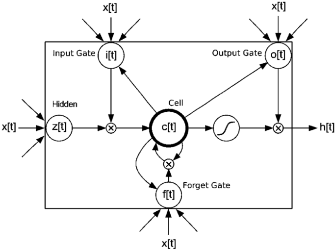
LSTM. Long short-term memory
Figure 6 
Predicting with LSTM. The LSTM model for predicting a lifestyle to trajectory. A one-hot vector has zeros for all trajectories except the specific trajectory (which is one)
-
BLSTM: Word embedding layer → Dropout → BLSTM layer → Dropout (see Fig. 7).
Figure 7 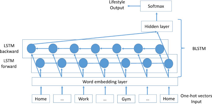
Predicting with BLSTM. The BLSTM model for predicting a lifestyle to trajectory. A one-hot vector has zeros for all trajectories except the specific trajectory (which is one)
-
CNN: Word embedding layer → Dropout → CNN and max pooling layer → Dropout → Neuron layer (see Fig. 8).
Figure 8 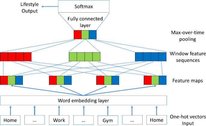
Predicting with CNN. The CNN model for predicting a lifestyle to trajectory. A one-hot vector has zeros for all trajectories except the specific trajectory (which is one). Each feature in a feature map is represented in a different color (could have more than three features)
-
CLSTM: Word embedding layer → Dropout → CNN and max pooling layer → Dropout → LSTM layer → Dropout (see Fig. 9).
Figure 9 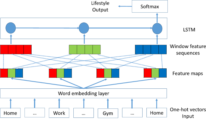
Predicting with CLSTM. The CLSTM model for predicting a lifestyle to trajectory. A one-hot vector has zeros for all trajectories except the specific trajectory (which is one). Each feature in a feature map is represented in a different color (could have more than three features)
-
CBLSTM: Word embedding layer → Dropout → CNN and max pooling layer → Dropout → BLSTM layer → Dropout (see Fig. 10).
Figure 10 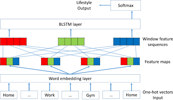
Predicting with CBLSTM. The CBLSTM model for predicting a lifestyle to trajectory. A one-hot vector has zeros for all trajectories except the specific trajectory (which is one). Each feature in a feature map is represented in a different color (could have more than three features)


In the next sections, we will give explanations about the RNN-based and CNN models.
4.1.1 LSTM
RNNs are a family of models which are able to capture time dynamics. In theory, RNNs are capable of capturing long-distance dependencies; however in practice, they fail due to the gradient vanishing problem [39].
LSTMs [40] are variants of RNNs which are designed to cope with the gradient vanishing problem. The LSTM unit (Fig. 5) has three multiplicative gates which control the proportions of information to forget and pass on to the next time step. Formally, in time t, the formulas to update an LSTM unit are [for the input gate (i), forget gate (f), and output gate (o)]:
where σ is the element-wise sigmoid function, ⊙ is the element-wise product, \(x_{t}\) is the input vector (e.g., word embedding) at time t, \(\boldsymbol{i}_{t}\) is the input gate vector which acquires new information, \(\boldsymbol{f}_{t}\) is the forget gate vector which remembers old information, \(\boldsymbol{o}_{t}\) is the output gate vector which is the output candidate, \(\tilde{\boldsymbol{c}}_{t}\) is in the tanh layer which creates a vector of new candidate values that can be added to the state if the input gate vector (\(\boldsymbol{i}_{t}\)) is larger than the forget gate vector (\(\boldsymbol{f}_{t}\)), \(\boldsymbol{c}_{t}\) is the cell state vector, and \(\boldsymbol {h}_{t}\) is the hidden state vector (also called the output). We put the cell state through tanh to push the values to be between −1 and 1. All the state vectors are memory units, which store all the useful information at, and before, time t. \(\boldsymbol{U}_{i}\), \(\boldsymbol{U}_{f}\), \(\boldsymbol {U}_{c}\), and \(\boldsymbol{U}_{o}\) denote the weight matrices of different gates for input \(x_{t}\), and \(\boldsymbol{W}_{i}\), \(\boldsymbol{W}_{f}\), \(\boldsymbol{W}_{c}\), and \(\boldsymbol{W}_{o}\) are the weight matrices for the hidden state \(\boldsymbol{h}_{t}\). \(\boldsymbol{b}_{i}\), \(\boldsymbol{b}_{f}\), \(\boldsymbol{b}_{c}\), and \(\boldsymbol{b}_{o}\) denote the bias vectors.
4.1.2 BLSTM
An LSTM remembers information only from the past/left of a sequence. In our study, when the whole trajectory exists (but not its corresponding lifestyle, which we wish to predict), we can also employ the future/right of a sequence. Dyer [41] suggested an elegant solution—bi-directional LSTM (BLSTM)—whose effectiveness was proven in previous work. The idea is to present each part of a sequence, one forward and one backward, for two different LSTM memory units. One should capture the past, and one the future. Then the two memory units are concatenated to one output.
4.1.3 CNN
We use CNN [42] to identify high-frequency sub-sequences of co-occurring POIs in the trajectories (i.e., mobility patterns), which are valuable for lifestyle prediction. Using a filter \(\boldsymbol{W} \in \mathbb{R}^{h \times k}\) of height h and width k as the length of the POI vector, a convolution operation on h consecutive POI vectors starting from the tth POI outputs a scalar feature
where \(\boldsymbol{X}_{t:t+h-1} \in\mathbb{R}^{k \times n}\) is a POI sequence matrix whose ith column is \(x_{i} \in\mathbb{R}^{k}\), e.g., a specific POI vector; n is the length of the trajectory; and \(b \in \mathbb{R}\) is a bias. The symbol • refers to the dot product, and \(\mathrm{Re}LU(\cdot)\) is an element-wise rectified linear unit function.
In this study, we checked the convolution operation with m different filters and denoted resulting features such as \(\boldsymbol{c}_{t} \in\mathbb {R}^{n-h-1}\), each of whose dimensions comes from a distinct filter. We repeated the convolution operations for each window of h consecutive POIs in the trajectory and obtained \(\boldsymbol{c}_{1:n-h+1}\). The trajectory representation is computed in the max pooling layer, \(\boldsymbol{s} \in\mathbb {R}^{n-h-1}\), where the element-wise maximum of \(\boldsymbol{c}_{1:n-h+1}\) is the output of the max pooling layer.
4.1.4 Dropout
Srivastava et al. [43] suggested a simple regularization technique named “Dropout” to solve the overfitting problem and to improve the performance of the NN. It randomly chooses units to drop out and removes them from the layer temporarily. In each training stage, each node (together with its incoming and outgoing edges) is either “dropped out” of the net with probability \(1-p\) or kept with probability p. Training at this stage is only of the reduced network. During the test, the removed nodes are reinserted into the network with their original weights.
4.2 Optimization of models for predicting lifestyles
The parameters of all the architectures were optimized using 5-fold cross-validation (CV5). We created five folds from all the users’ trajectories: three folds used for the training set, one fold used for the validation set, and one fold for the test set, and changed the roles of the folds five times. It is important to note that the CV5 performs on approximately 12K unique trajectories—every trajectory in the training set was different from every other. Also, the trajectories in the validation and test sets were not seen during training.
In the next sections, we describe how we found the best parameters for the different models.
4.2.1 NN optimization
For each NN layer or mechanism (e.g., word embedding, dropout, RNN/LSTM/BLSTM, and CNN; see Sect. 4.1), we optimized its different parameters. In the word embedding layer, the parameter was the hidden node number in the hidden layer, which was checked between 500 and 1300 with a 100 hidden-node jump. In the CNN layer, the parameters were the filter size, which was evaluated between two and seven with a one-step jump, and the number of filters, which was checked between 500 and 1300 with a 100 hidden-node jump. The max pooling layer was set to be global. Last, in the RNN/LSTM layer (used by all LSTM variants; Sect. 4.1), the memory unit number was tested between 500 and 1300 with a 100 hidden-node jump. For all the models, we used 35 epochs and 64 trajectories as the batch size. For each of the evaluated parameters, its best value was selected using the validation set, as described in Sect. 5.
4.2.2 Optimization of the traditional models
We compared the six NN system architectures (Sect. 4.1) with traditional models: NBC, support vector machine (SVM), and HMM, with respect to accuracy and generalizability. The preprocessing stage of representing trajectories using TFs for the SVM is similar to that for the NBC (Sect. 3.2). However, since some terms can be more common than others in trajectories (e.g., {home, work, work} is more common than {school, work, gym}), and thus can be less effective in distinguishing trajectories (and lifestyles), we weighted terms by the inverse of their frequency using the inverse document frequency (IDF) [44] for both the NBC and SVM (where whether to use IDF or not was a model’s parameter to evaluate).
We tested four SVM models: linear SVM (LSVM), radial basis kernel function SVM (RSVM), polynomial kernel function SVM (PSVM), and linear support vector classification (SVC). A parameter to evaluate for the SVM models was the cost-function term C. For all SVM-based algorithms, C was checked between 0.2 and one with a 0.2-step jump. Other parameters tested for the NBC and SVM-based algorithms were n for the n-gram, which was checked between two and fourteen with a two-step jump.
In addition, we tested several HMM models, one for each lifestyle (a lifestyle was found as explained in Sect. 3.8). The parameters of the model were the number of hidden states, where values checked were between ten and 40 with a ten hidden-state jump, and the convergence threshold of the expectation maximization (EM) algorithm, which was examined in between 0.01 and 0.1 with a 0.01-step jump. In the test, we tested each HMM model (for a different lifestyle) on each trajectory and calculated the log-likelihood of the trajectory given the model. The lifestyle was predicted by the HMM model that had the best log-likelihood on this trajectory.
For all algorithms, the best parameter valuess were determined by the validation set, as described in Sect. 5.
5 Results
For training the different models, we implemented the NNs with different Python packages and different computation resources: For the NNs that were used to predict lifestyles, we used Keras [45] based on TensorFlow [46]. The computations for a single model were run on a GeForce GTX 1080 GPU. For the traditional models that were used to predict the lifestyles, we used Scikit-learn [47]. The computations for a single model were run on an Intel core I7-6800K CPU 3.4 GHz × 12.
We used a “society” of 38 users for whom data is presented in Table 2. We recruited the users from three different sources: (1) The Upwork–freelancer platform (http://www.upwork.com). (2) Academic institutes in Israel, and (3) Friends and family. We obtained Ethical Committee approval from the Ben Gurion University of the Negev and Sapir Academic College. All users signed a consent form. The users’ distribution is as follows:
-
Recruited sources: Upwork: 2; Academic institutes: 18; Friends and family: 18.
-
Gender: Female: 15; Male: 23.
-
Age: Between 20–30: 21; Between 30–40: 10; Between 40–60: 5; Over 60: 2.
-
Profession: Undergraduate students: 16; Graduate students: 7; Engineers: 4, Freelancers: 3; Others: 8.
-
Status: Married: 15; In relationship: 4; Single: 19.
As can be seen, most of the users are between the age of 20 and 30 years old, most of them are students at some level of degree and are single. This user demographic could have a bias on the models’ predictions, because such users have a high level of uncertainty.
For identifying lifestyles by trajectory, we applied t-SNE to 1865 two-consecutive week periods for all the users, with 11,350 unique trajectories in those weeks. To predict a lifestyle by trajectory, we used the unique trajectories of all the users. We clustered the trajectories (Sect. 3.5) into 3000 different clusters.
As we can see in Fig. 11(A), the t-SNE projection created groups of trajectories, i.e., similar trajectories are close to one another, and dissimilar trajectories are more distant from each other. We checked a changing lifestyle number between 2 and 80 on the t-SNE projection with hierarchical clustering. In Fig. 11(B), we can see the potential candidates of the lifestyle number, which are 5, 14, and around 18. The likely candidates were chosen by the peaks of the Calinski–Harabaz index. We decided the lifestyle number as 14 because less than this number was not interesting enough, and as we see in Fig. 11(A), there are more than five groups of trajectories. We did not choose 18 lifestyles because we did not have enough data to support our models, especially for the deep neural networks. Future studies could examine more significant numbers than 14 conditioned on data availability.

Preprocessing results. Results for identifying lifestyles
Table 3 and Fig. 12 show trajectory distribution over the 14 lifestyles that were identified by the hierarchical clustering with the Euclidean distance on the t-SNE projection. We can see that most users (almost 70% of them) have seven or less lifestyles, and more than 30% of the users have three or less lifestyles.

Trajectory distribution over lifestyles
In predicting lifestyles, we used two architectures; One for predicting a lifestyle for a never-seen-before trajectory and another for predicting a lifestyle for a never-seen-before user. The first architecture was implemented using CV5 over all the unique trajectories to optimize/maximize the models’ hyper-parameters based on the accuracy score. The second architecture was implemented using a leave-one-out methodology over the users using the hyper-parameters from the first architecture, and different performance measures were calculated for the prediction models alternatively trained using data of all but a single user, when that user is tested.
In the next section, we describe the performance measures that evaluated the prediction of lifestyle for a trajectory.
5.1 Performance measures for lifestyle prediction
Although our task is (lifestyle) multiclass classification, to simplify the explanation and notation, we introduce our performance measures using a confusion matrix for the binary case (Table 4).
Accuracy. Accuracy is calculated as: \(\frac{TP + TN}{\sum{\text{Total population}}}\) (Table 4), and is between 0 and 1, where 1 is a perfect prediction, and 0 is the worst prediction.
Recall. Recall is calculated as: \(\frac{TP}{TP + FN}\) (Table 4), and is between 0 and 1, where 1 indicates the model has no false negatives, and 0 means all positive examples are misclassified.
Precision. Precision is calculated as: \(\frac{TP}{TP + FP}\), and is between 0 and 1, where 1 indicates the model has no false positives, and 0 means all positive examples are misclassified.
F1 score. The f1 score is calculated as: \(2 \cdot\frac{\text{Precision} \cdot \text{Recall}}{\text{Precision} + \text{Recall}}\), and is between 0 and 1, where 1 shows perfect precision and recall, and 0 shows that either one or both of the measures are 0.
Cohen’s Kappa score. The Cohen’s Kappa score is calculated in several steps: (1) \(P_{0} = \frac {TP +TN}{\sum{\text{Total population}}}\), (2) \(P_{\mathrm{Yes}} = \frac{TP + FN}{\sum {\text{Total population}}} \cdot\frac{TP + FP}{\sum{\text{Total population}}}\), (3) \(P_{\mathrm{No}} = \frac{FP + TN}{\sum{\text{Total population}}} \cdot\frac{FN+ TN}{\sum{\text{Total population}}}\), 4) \(P_{e} = P_{\mathrm{Yes}} + P_{\mathrm{No}}\), and finally, \(\kappa=(P_{0} - P_{e}) / (1 - P_{e})\). The Cohen’s Kappa score is between 0 and 1, where 1 indicates complete agreement between two raters who each classify items into mutually exclusive categories, and 0 indicates complete disagreement.
Jaccard similarity. The Jaccard similarity (intersection over union) is calculated as: \(\frac{TP}{TP + FP + FN}\), and is between 0 and 1, where 1 indicates all examples were predicted accurately, and 0 indicates none of the positive examples was predicted correctly as positive.
Hamming loss. The Hamming loss is calculated as: \(\frac{FP + FN}{\sum{\text{Total population}}}\), and is between 0 and 1, where 0 indicates no examples are incorrectly predicted, and 1 indicates all examples are incorrectly predicted.
5.2 CV5 results
Table 5 shows the best hyper-parameters for the tested models based on the validation sets in the CV5 experiment over all unique trajectories of all users together. These hyper-parameters were chosen from wide and substantial sets of ranges. As can be seen for the embedding layer, the hidden node number “Embed” of the hidden layer is much greater than 34, which is the number of different POIs (our vocabulary of POIs for all users). Also for the RNN and all its variations, the number of memory units is much larger than 24, the trajectory size. This evidence is supported by Livni et al. [48], who showed that when the network is over-specified, i.e., it is larger than needed, the NN results improve much more.
Table 6 and Fig. 13 show that the average accuracy of the best model, CLSTM, in the CV5 experiment is 52%. This accuracy is pretty good because the dependent variable, lifestyle, has 14 classes, and if we were predicting a lifestyle for a trajectory based on the a-priori probabilities (Table 3), we would have achieved accuracy of approximately 12%, which is more than four times less than that of the CLSTM. Therefore, we believe the CLSTM has identified meaningful mobility patterns to distinguish the users and predicted them to their lifestyles relatively correctly. Also all the other performance measures peak for CLSTM. The performance measures of the traditional models are poor, e.g., showing accuracy similar to the a-priori probability of the majority class.

Performance measures over CV5. Performance measures averaged over all trajectories of all users in a CV5 experiment
5.3 Leave-one-out results
Table 7 and Fig. 14 show that also in the leave-one-out experiment, when 38 times another user is tested on a model trained using the other 37 users, the CLSTM is the best model with respect to all performance measures. Its results for the leave-one-out experiment are almost identical to those for the CV5 experiment, except for the recall, precision, and thus also the f1, measures. For these three performance measures, the results in the CV5 experiment are better than in the leave-one-out experiment, especially for CLSTM. We attribute this result to the variability among the users that affect the leave-one-out setting more than the CV5 one. Thus, also the standard deviations (STD) of the measures (not shown) over the CV5 experiment are smaller than for the leave-one-out setting. This is because when we identify lifestyles and predict lifestyles for trajectories using all data, we smooth the noise over the users’ data, and as a result, the STD is smaller than if we were using the leave-one-out setting. Also here, the performance measures of the traditional models are poor.

Performance measures over leave-one-out. Performance measures averaged over 38 users in a leave-one-out experiment
Table 8 shows some statistics (numbers of trajectories, lifestyles, and POIs) about the data of each of the 38 users and the accuracy for each user of the CLSTM model, which is the best model on average over the users. We see that the number of lifestyles for all users is quite similar (11–14), and that the number of trajectories usually increases with the number of POIs a user has. Accuracy performance varies dramatically among users, from a low value of around 0.3 to a very high one of around 0.8, and even 0.86, but cannot be related to the numbers of trajectories, lifestyles, or POIs, and thus it is attributed only to the complexity of the mobility patterns a user has.
Using [49], we compared all models using the Friedman and Nemenyi post-hoc tests [50], with a significance level of 5%, on the accuracy measure over the 38 users (this cannot be done with CV5 that has only five data sets). We chose to use the Friedman test because the accuracy is not distributed normally, the number of the models is greater than two, and the number of datasets is greater than twice the number of the models (38 datasets/users vs. 12 models), as required for a Friedman test. For the accuracy measure, the null hypothesis, H0, of the Friedman test was rejected with a \({p}\text{-value}=0\), meaning that there are differences among the models. Table 9 shows that according to the Friedman test, the best ranked model is CLSTM, and according to the Nemenyi post-hoc test, this model is identical to the LSTM, BLSTM, and CBLSTM because they are all in the same group. This group of the LSTM models is superior to, and well separated from, all other models. These results demonstrate the strength of the convolution and LSTM layers in significantly improving the prediction results.
6 Summary and discussion
In this study, we presented a full framework for identifying and predicting lifestyles from human mobility patterns represented in, and extracted from, trajectories of movement. We generalized a previous study that modeled only individual users to models for a “society” of people and thereby could identify and predict social lifestyles. We developed and applied a system of NNs: (1) to embed POI-based daily trajectories that always appear together with others in consecutive weeks in lifestyles, (2) to identify high-frequency sub-sequences of co-occurring POIs (mobility patterns) in the embedded trajectories, and (3) to train a model to predict a social lifestyle for a trajectory never-seen-before.
Comparing Table 8 and Table 2, and adding some background knowledge we have about most of the 38 users, we can conclude that when the mobility patterns of a user have a low level of “uncertainty,” e.g., his routine is stable, the CLSTM model has a high level of accuracy. We identify three groups of users according to the variability/uncertainty in their mobility patterns. Those with stationary mobility patterns; those with changing mobility patterns, but still some stationarity; and those with mobility patterns that change very frequently.
For example, User 14 is a 60-year old pensioner (Table 2) with a very stable life. In most weeks, she goes to the market on Tuesday, and on specific days of the month she goes to the theater, hair stylist, and several social events. This user belongs to the first group of users, and the CLSTM model was very accurate (with 0.86 accuracy) for her (Table 8). User 26 is an M.Sc. student, who has some routine in his life as being student, but also has non-regular mobility patterns when he goes to the market, does his volunteering duties, and attends some social group activities. This user belongs to the second group of users, and the CLSTM model was moderately accurate for him (with 0.54 accuracy). Finally, User 21 is a freelancer with a low level of stationarity in his mobility patterns. Every week and even every day, he has a new project in a new location, which causes his routine to change very often. This user belongs to the third group, and the model predicts his lifestyles poorly (with 0.27 accuracy).
7 Conclusions
Using a system of NN models, we can (1) embed in social lifestyles daily trajectories that always appear together with others in consecutive weeks in cellular data of a society of people, (2) identify mobility patterns in the embedded trajectory, and (3) train a model to predict a social lifestyle based on mobility-pattern representation of a trajectory.
Our system shows accuracy and generalizability in lifestyle identification and prediction (both for a novel trajectory and a novel user) that are superior to those shown by state-of-the-art algorithms.
8 Future work
Future work can optimize finding the numbers of trajectory clusters and lifestyles using ideas recently published [51, 52]. Also, lifestyle prediction can be improved by making the LSTM more efficient [53].
Prediction of lifestyles can be improved also by adding to the model a latent variable to represent the “uncertainty” in the lifestyle, thereby helping the model to be more accurate by trying to explain part of the noise in each user’s mobility pattern using this latent variable.
Another avenue for possible research is in understanding the relations between types of POIs and the ability to predict the next POI. The current research demonstrated the accuracy of the LSTM as a suitable prediction model for the next POI; thus, by computing a confusion matrix among all POI types, we could check for which POI types the model is correct or incorrect, and try to improve its prediction in the latter case.
Abbreviations
- POI :
-
Point Of Interest
- LS :
-
LifeStyle
- NLP :
-
Natural Language Processing
- LDA :
-
Latent Dirichlet Allocation
- TF :
-
Term FSrequency
- IDF :
-
Inverse Document Frequency
- CBOW :
-
Continuous Bag-Of-Words
- NEG :
-
Negative Sampling
- NCE :
-
Noise Contrastive Estimation
- t-SNE :
-
t-Distributed Stochastic Neighbor Embedding
- NN :
-
Neural Network
- CNN :
-
Convolutional Neural Network
- RNN :
-
Recurrent Neural Network
- LSTM :
-
Long Short-term Memory
- BLSTM :
-
Bi-directional Long Short-term Memory
- CLSTM :
-
Convolutional Neural Network and Long Short-term Memory
- CBLSTM :
-
Convolutional Neural Network and Bi-directional Long Short-term Memory
- CV :
-
Cross Validation
- HMM :
-
Hidden Markov Model
- SVM :
-
Support Vector Machine
- LSVM :
-
Linear Support Vector Machine
- RSVM :
-
Radial basis Support Vector Machine
- PSVM :
-
Polynomial Support Vector Machine
- SVC :
-
Linear Support Vector Classification
- EM :
-
Expectation Maximization
- NB :
-
Naive Bayes
- TP :
-
True Positive
- FP :
-
False Positive
- TN :
-
True Negative
- FN :
-
False Negative
- STD :
-
STandard Deviations
References
Ben Zion E, Lerner B (2017) Learning human behaviors and lifestyle by capturing temporal relations in mobility patterns. In: European symposium on artificial neural networks, computational intelligence and machine learning, XXV. European Neural Network Society-ENNS, Bruges
Mikolov T, Chen K, Corrado G, Dean J (2013) Efficient estimation of word representations in vector space. arXiv:1301.3781
van der Maaten L, Hinton G (2008) Visualizing data using t-SNE. J Mach Learn Res 9:2579–2605
Xing Z, Pei J, Keogh E (2010) A brief survey on sequence classification. ACM SIGKDD Explor Newsl 12(1):40–48
Ma X, Hovy E (2016) End-to-end sequence labeling via bi-directional LSTM-CNNs-CRF. arXiv:1603.01354
Dietterich TG (2002) Machine learning for sequential data: a review. In: Joint IAPR international workshops on statistical techniques in pattern recognition (SPR) and structural and syntactic pattern recognition (SSPR), Windsor, ON, Canada, pp 15–30
Rong X (2014) Word2vec parameter learning explained. arXiv:1411.2738
Soh W-S, Kim HS (2003) QoS provisioning in cellular networks based on mobility prediction techniques. IEEE Commun Mag 41(1):86–92. https://doi.org/10.1109/MCOM.2003.1166661
Ashbrook D, Starner T (2003) Using GPS to learn significant locations and predict movement across multiple users. Pers Ubiquitous Comput 7(5):275–286. https://doi.org/10.1007/s00779-003-0240-0
Choudhury T, Hightower J, Lamarca A, Legrand L, Rahimi A, Rea A, Hemingway B, Koscher K, Landay J, Lester J, Wyatt D (2008) An embedded activity recognition system. IEEE Pervasive Comput 7(2):32–41. https://doi.org/10.1109/MPRV.2008.39
Munguia E, Intille SS, Larson K (2004) Activity recognition in the home using simple and ubiquitous sensors. In: Pervasive computing, vol 3001. Linz, Vienna, pp 158–175. https://doi.org/10.1007/b96922
Wyatt D, Philipose M, Choudhury T (2005) Unsupervised activity recognition using automatically mined common sense. In: Sensors, Pittsburgh, PA, USA, vol 20, pp 21–27. http://citeseerx.ist.psu.edu/viewdoc/summary?doi=10.1.1.61.9138
Liao L, Fox D, Kautz H (2007) Extracting places and activities from GPS traces using hierarchical conditional random fields. Int J Robot Res 26(1):119–134
Liao L, Fox D, Kautz H (2006) Location-based activity recognition using relational Markov networks. In: Proceedings of the 20th annual conference on neural information processing systems (NIPS), Vancouver, Canada, pp 787–794. https://doi.org/10.1007/b96922
Eagle N, Pentland AS (2009) Eigenbehaviors: identifying structure in routine. Behav Ecol Sociobiol 63(7):1057–1066. https://doi.org/10.1007/s00265-009-0739-0
Khoroshevsky F, Lerner B (2017) Human mobility-pattern discovery and next-place prediction from GPS data. In: IAPR workshop on multimodal pattern recognition of social signals in human-computer interaction. Springer, Berlin, pp 24–35
Toch E, Lerner B, Ben Zion E, Ben-Gal I (2018) Analyzing large-scale human mobility data: a survey of machine learning methods and applications. Knowledge and Information System, 1–23
Blei DM, Ng AY, Jordan MI (2003) Latent Dirichlet allocation. J Mach Learn Res 3:993–1022
Mikolov T, Le QV, Sutskever I (2013) Exploiting similarities among languages for machine translation. arXiv:1309.4168
Mikolov T, Yih W-t, Zweig G (2013) Representations, linguistic regularities in continuous space word. In: 013 conference of the North American chapter of the association for computational linguistics: human language technologies, vol 13. Atlanta, GA, USA, pp 746–751
Perozzi B, Al-Rfou R, Skiena S (2014) Deepwalk: online learning of social representations. In: Proceedings of the 20th ACM SIGKDD international conference on knowledge discovery and data mining. New York, NY, USA, pp 701–710
Tang D, Qin B, Liu T, Yang Y (2015) User modeling with neural network for review rating prediction. In: Proceedings of the twenty-fourth international joint conference on artificial intelligence, Buenos Aires, Argentina, pp 1340–1346
Tang D, Qin B, Liu T (2015) Learning semantic representations of users and products for document level sentiment classification. In: 53th annual meeting of the association for computational linguistics-ACL 2015, Beijing, China, pp 1014–1023
Grbovic M, Radosavljevic V, Djuric N, Bhamidipati N, Savla J, Bhagwan V, Sharp D (2015) E-commerce in your inbox: product recommendations at scale. In: Proceedings of the 21th ACM SIGKDD international conference on knowledge discovery and data mining, Sydney, NSW, Australia, pp 1809–1818
Ozsoy MG (2016) From word embeddings to item recommendation. arXiv:1601.01356
Ying JJ-C, Lee W-C, Tseng VS (2013) Mining geographic-temporal-semantic patterns in trajectories for location prediction. ACM Trans Intell Syst Technol 5(1):2
Zhao S, Zhao T, King I, Lyu MR (2016) GT-SEER: geo-temporal sequential embedding rank for point-of-interest Recommendation. arXiv:1606.05859
Le QV, Mikolov T (2014) Distributed representations of sentences and documents. In: International conference on machine learning, Beijing, China, pp 1188–1196
Liu P, Qiu X, Huang X (2015) Learning context-sensitive word embeddings with neural tensor skip-gram model. In: Proceedings of the twenty-fourth international joint conference on artificial intelligence, Buenos Aires, Argentina, pp 1284–1290
Liu Y, Liu Z, Chua T-S, Sun M (2015) Topical word embeddings. In: Twenty-ninth AAAI conference on artificial intelligence, Austin, TX, USA, pp 2418–2424
Gao Q, Zhou F, Zhang K, Trajcevski G, Luo X, Zhang F (2017) Identifying human mobility via trajectory embeddings. In: Proceedings of the 26th international joint conference on artificial intelligence. AAAI Press, Menlo Park, pp 1689–1695
GoogleMaps (2016) https://www.google.co.il/maps/
Asgari E, Mofrad MR (2015) Continuous distributed representation of biological sequences for deep proteomics and genomics. PLoS ONE 10(11):0141287
Banerjee I, Chen MC, Lungren MP, Rubin DL (2017) Radiology report annotation using intelligent word embeddings: applied to multi-institutional chest CT cohort. Journal of Biomedical Informatics
Gutmann M, Hyvärinen A (2010) Noise-contrastive estimation: a new estimation principle for unnormalized statistical models. In: Thirteenth international conference on artificial intelligence and statistics, AISTATS, vol 1. Sardinia, Italy, p 6
Jamieson AR, Giger ML, Drukker K, Li H, Yuan Y, Bhooshan N (2010) Exploring nonlinear feature space dimension reduction and data representation in breast CADx with Laplacian eigenmaps and t-SNE. Med Phys 37(1):339–351
Hamel P, Eck D (2010) Learning features from music audio with deep belief networks. In: ISMIR, Utrecht, The Netherlands, pp 339–344
Wallach I, Lilien R (2009) The protein–small-molecule database, a non-redundant structural resource for the analysis of protein-ligand binding. Bioinformatics 25(5):615–620
Bengio Y, Simard P, Frasconi P (1994) Learning long-term dependencies with gradient descent is difficult. IEEE Trans Neural Netw 5(2):157–166
Hochreiter S, Schmidhuber J (1997) Long short-term memory. Neural Comput 9(8):1735–1780
Dyer C, Ballesteros M, Ling W, Matthews A, Smith NA (2015) Transition-based dependency parsing with stack long short-term memory. arXiv:1505.08075
Kim Y (2014) Convolutional neural networks for sentence classification. arXiv:1408.5882
Srivastava N, Hinton GE, Krizhevsky A, Sutskever I, Salakhutdinov R (2014) Dropout: a simple way to prevent neural networks from overfitting. J Mach Learn Res 15(1):1929–1958
Robertson S (2004) Understanding inverse document frequency: on theoretical arguments for IDF. J Doc 60(5):503–520
Chollet F (2015) Keras. GitHub
Abadi M, Agarwal A, Barham P, Brevdo E, Chen Z, Citro C, Corrado GS, Davis A, Dean J, Devin M, Ghemawat S, Goodfellow I, Harp A, Irving G, Isard M, Jia Y, Jozefowicz R, Kaiser L, Kudlur M, Levenberg J, Mané D, Monga R, Moore S, Murray D, Olah C, Schuster M, Shlens J, Steiner B, Sutskever I, Talwar K, Tucker P, Vanhoucke V, Vasudevan V, Viégas F, Vinyals O, Warden P, Wattenberg M, Wicke M, Yu Y, Zheng X (2015) TensorFlow: large-scale machine learning on heterogeneous systems. Software available from tensorflow.org. https://www.tensorflow.org/
Pedregosa F, Varoquaux G, Gramfort A, Michel V, Thirion B, Grisel O, Blondel M, Prettenhofer P, Weiss R, Dubourg V et al. (2011) Scikit-learn: machine learning in python. J Mach Learn Res 12:2825–2830
Livni R, Shalev-Shwartz S, Shamir O (2014) On the computational efficiency of training neural networks. In: Advances in neural information processing systems, Montreal, QC, Canada, pp 855–863
Rodríguez-Fdez I, Canosa A, Mucientes M, Bugarín A (2015) STAC: a web platform for the comparison of algorithms using statistical tests. In: Proceedings of the 2015 IEEE international conference on fuzzy systems (FUZZ-IEEE)
Demšar J (2006) Statistical comparisons of classifiers over multiple data sets. J Mach Learn Res 7:1–30
Guo G, Chen L, Ye Y, Jiang Q (2017) Cluster validation method for determining the number of clusters in categorical sequences. IEEE Trans Neural Netw Learn Syst 28(12):2936–2948
Zhou S, Xu Z, Liu F (2017) Method for determining the optimal number of clusters based on agglomerative hierarchical clustering. IEEE Trans Neural Netw Learn Syst 28(12):3007–3017
He Z, Gao S, Xiao L, Barber D (2017) Wider and deeper, cheaper and faster: tensorized LSTMs for sequence learning. In: Advances in neural information processing systems, pp 1–11
Acknowledgements
We thank Orit Zehavi for her help in data preparation including the creation of a list of common semantic POIs.
Availability of data and materials
The code for the algorithm and data sets used in our experiments are available online .
Authors’ information
Eyal Ben Zion received his Ph.D. from the Industrial Engineering and Management (IEM) Department at Ben–Gurion University of the Negev under the supervision of Boaz Lerner in February 2018. In his dissertation, he studied machine learning methods to analyze, learn, identify, and predict human mobility patterns from data. He holds a BSc and an MSc also from the IEM Department at Ben–Gurion University. Today, Eyal works for Shoodoo Analytics LTD as a senior data scientist. In his work, he supervises the building of data science products. Boaz Lerner is a Professor of Machine Learning in the Industrial Engineering and Management (IEM) Department at Ben–Gurion University of the Negev. He holds a BA (Physics and Mathematics), MSc (Electro-Optical Engineering), and PhD (Computer Engineering) from the Hebrew University, Tel-Aviv University, and Ben–Gurion University, respectively. Before joining IEM, he did research at Aston and Cambridge Universities (UK). During the last 25 years, Lerner has been investigating, developing, teaching, and consulting in machine learning and data mining. In 2007, he established and has since headed the Machine Learning and Data Mining Lab at IEM in which numerous projects for different agencies, authorities, and companies have been undertaken. Lerner has supervised nearly 50 graduate students and has published around 100 papers in journals and conference proceedings.
Funding
Not applicable.
Author information
Authors and Affiliations
Contributions
EBZ collected the data, designed and trained the models, performed the experiments, interviewed the users, and wrote the paper. BL supervised all these stages of the work and contributed to the writing. All authors read and approved the final manuscript.
Corresponding author
Ethics declarations
Competing interests
The authors declare that they have no competing interests.
Additional information
Publisher’s Note
Springer Nature remains neutral with regard to jurisdictional claims in published maps and institutional affiliations.
Rights and permissions
Open Access This article is distributed under the terms of the Creative Commons Attribution 4.0 International License (http://creativecommons.org/licenses/by/4.0/), which permits unrestricted use, distribution, and reproduction in any medium, provided you give appropriate credit to the original author(s) and the source, provide a link to the Creative Commons license, and indicate if changes were made.
About this article

Cite this article
Ben Zion, E., Lerner, B. Identifying and predicting social lifestyles in people’s trajectories by neural networks. EPJ Data Sci. 7, 45 (2018). https://doi.org/10.1140/epjds/s13688-018-0173-5
Received:
Accepted:
Published:
DOI: https://doi.org/10.1140/epjds/s13688-018-0173-5