- Regular article
- Open access
- Published:
Crime event prediction with dynamic features
EPJ Data Science volume 7, Article number: 43 (2018)
Abstract
Nowadays, Location-Based Social Networks (LBSN) collect a vast range of information which can help us to understand the regional dynamics (i.e. human mobility) across an entire city. LBSN provides unprecedented opportunities to tackle various social problems. In this work, we explore dynamic features derived from Foursquare check-in data in short-term crime event prediction with fine spatio-temporal granularity. While crime event prediction has been investigated widely due to its social importance, its success rate is far from satisfactory. The existing studies rely on relatively static features such as regional characteristics, demographic information and the topics obtained from tweets but very few studies focus on exploring human mobility through social media. In this study, we identify a number of dynamic features based on the research findings in Criminology, and report their correlations with different types of crime events. In particular, we observe that some types of crime events are more highly correlated to the dynamic features, e.g., Theft, Drug Offence, Fraud, Unlawful Entry and Assault than others e.g. Traffic Related Offence.
A key challenge of the research is that the dynamic information is very sparse compared to the relatively static information. To address this issue, we develop a matrix factorization based approach to estimate the missing dynamic features across the city. Interestingly, the estimated dynamic features still maintain the correlation with crime occurrence across different types. We evaluate the proposed methods in different time intervals. The results verify that the crime prediction performance can be significantly improved with the inclusion of dynamic features across different types of crime events.
1 Introduction
Crime event prediction is important to crime prevention in the society by helping the law enforcement agencies to design optimal patrol strategies. Reduction of crime events will benefit society in numerous ways. It will increase the public safety and decrease the economic loss. However, crime event prediction is a challenging task [1]. The spatial and temporal distributions of crime events differ from one type to the other. As shown in Fig. 1, we can observe the difference in the spatial distribution of three different types of crime event, i.e., Theft, Drug Offence, and Assault respectively in Brisbane. Many factors are relevant to the possibility that a particular type of crime event is going to occur in a region in the near future. These include demographics, the distribution of different types of services, crime history, human mobility and so on.

Spatial distribution of different types of crime event in Brisbane
Traditionally, crime event prediction uses the historical patterns of crime events, the information collected from geographic information systems (GIS) and demographic variables, e.g. sex, income, age, and race and so on. But these variables are almost constant or only change slowly over time. Therefore, they do not capture the short-term variations of the factors which are relevant to the occurrence of crime events [2]. With the widespread use of social media such as Twitter and Foursquare in the last decade, large volumes of information have been generated which provide unprecedented opportunities to capture the city dynamics, i.e. human mobility across a city [3]. A few researchers take advantage of Twitter data to assist crime event prediction [4–6]. They capture the sentiments of neighborhoods by topic analysis of Twitter data. While the sentiments change over time, it typically takes a relatively long time to identify the change. According to some urban research [7], the diversity of visitors to a location and associated influences over time are directly relevant to an area’s safety and one can obtain such high dynamic information on human mobility from LBSN data. But they are ignored largely in crime event prediction. This work attempts to fill the gap.
For a given city with R regions (known as meshblocks or census regions), we aim to identify the regions where a certain type of crime event will happen in the next time interval. Several types of crime event are studied including Theft, Unlawful Entry, Drug Offence, Traffic Related Offence, Fraud, and Assault. The criminal offence which includes the illegal taking of other persons belonging without consent to permanently or temporarily deprive the owner is defined as Theft. When a person enters a building (e.g. office, bank, shop etc.) with an intention to commit crime can be classified as Unlawful Entry. Drug Offence includes any form of sale, dealing, importing or exporting, manufacture or cultivation of illegal drugs or other substances. The offences which are related to most forms of road traffic, including pertaining to the licensing, registration, road worthiness or use of vehicles, bicycle offences, and pedestrian offences can be classified as Traffic Related Offence. According to the Queensland Police,Footnote 1 Fraud is a type of behavior towards a person or organization which is deceptive, dishonest, corrupt or unethical. All types of physical and mental harm towards a person are defined as Assault. This includes all types of physical contact with a person without their consent.
In this study, with an aim for short-term crime event prediction we partition a day into total eight intervals and each interval spans 3 hours. Crime prediction in finer temporal grain will help the police to design their patrol strategy dynamically and it will increase the probability to reduce crime rate more effectively. It is to be noted that the time span is independent of the methodology applied. User can change the interval span in different application scenarios. We derive a series of features and categorize them into four categories: historical, demographic, geographic and dynamic. We derive the historical features from the crime event records. They describe the density and trend of crime event in a region and the surrounding regions. The demographic features reflect the socio-economic conditions of residents in a region. The geographic features retain the information about the properties of venues in a region. While the crime event prediction has been studied by exploring historical, demographic, geographic features, the unique aspects of this work lies in the proposal of a series of dynamic features in crime event prediction. We extract the dynamic features from check-ins of Foursquare users. For a particular Foursquare user, the visiting history is associated with her/his habits and routines [8, 9]. According to routine activity theory, the opportunities for crime events are optimized in places where victims and offenders come together in greater concentrations [10, 11]. For example, a location with visitors from diverse backgrounds in a time interval is highly correlated with some types of crime event such as Theft; monitoring the fluctuation of visitor diversity at locations provides useful information to the crime event prediction. The contributions of this paper are summarized as follows:
-
This work systematically explores highly dynamic human mobility from Location-Based Social Network to lift the crime event prediction performance.
-
This work identifies a number of dynamic features derived from Foursquare check-ins based on the research findings in Criminology. On real data sets in Brisbane and New York City, we have conducted extensive tests with the widely used prediction models (including SVM, Random Forest, Neural Network, and Logistic Regression) and an ensemble model, and the widely used features (historical features, geographic features, demographic features) in existing crime event prediction studies. The prediction performance before and after adding the proposed dynamic features have been performed and compared. The test results demonstrate the improvement of prediction performance after adding dynamic features is considerable and statistically significant.
-
The dynamic features are highly sparse compared to the relatively static features. To handle this issue, we have developed a matrix factorization based approach to estimate the missing dynamic features across the city. Interestingly, the estimated dynamic features well retain the correlation with crime event occurrences of different types.
The rest of the paper is organized as follows. In Sect. 2, we briefly introduce the related work in crime event prediction. Section 3 describes the data sets used in this study. Section 4 discusses the details of the prediction features and shows the correlations between dynamic features and different types of crime event. In Sect. 5, the sparsity of dynamic features is addressed. The evaluation results on real data sets are reported in Sect. 6. Finally, this work is concluded in Sect. 7.
2 Related work
Predictive policing is defined as applications of statistical prediction methods which identify the likely targets to prevent crime events [12]. It allows police officers to design effective patrol strategies with limited resources. Crime Event Prediction has been studied widely using several types of information. The state-of-the-arts have generally explored relative static features including long-term historical information [1, 13], geographical information [14], and demographic information [14] in crime event prediction. This information changes slowly over time. So, it can’t capture the short-term variations in crime event occurrences. While the urban activities have argued that population diversity and visitors’ ratio contribute to an area’s safety [7, 15], they change frequently due to human mobility. In our study, we have exploited the human mobility data from foursquare to represent the human dynamics of a region for a short time period. Later, it has verified the impact of dynamic features on top of related constant features in short-term crime event prediction of various types. We have categorized the existing works into four following types.
2.1 Crime event prediction using historical information
Traditional methods for crime event prediction assume that crime events are most likely to happen in the vicinity of past crime events. For a given region, the historical data of a certain type of crime events is analyzed to predict the possibility of the crime event to happen in the near future (e.g. [1]). Various models have been developed over the past decade including regression model, machine learning techniques like Neural Networks, Support Vector Machine (SVM), One Nearest Neighbor (1NN), Decision Tree, Random Forest, and Ensemble Learning.
In [1], they focus on Burglary prediction. The city is divided using a grid. For each grid cell, the number of Burglary in the past is counted by month. They run several classifiers including 1NN, J48, SVM, Neural Network and Naive Bayes to predict the possibility of Burglary in the next month for each grid cell based on the crime historical data in this cell and neighboring cells. It shows J48, SVM, Neural Network always outperform the others and Neural Network often performs better than J48 and SVM. But this model solely depends on the past history of crime events in the vicinity.
In [16] and its extended version [13], the authors propose a Cluster-Confidence-Rate-Boosting algorithm (CCRBoost) which concurrently considers the spatial and temporal factors as well as the relevant types of crime event. For example, a type of crime event, e.g., Robbery, is used as an indicator of the relevant crime event to be predicted, e.g., Burglary. Different indicators of the same location in the same period of time are used to form a vector. Each vector has one class label which informs whether this location is a hot spot for the crime event to be predicted.
In [17], the authors use the theory of self-exciting point process (SEPP) method in crime prediction particularly in residential burglary prediction. SEPP is a popular approach for modeling space-time clustering of seismic activity. They demonstrate that a better prediction performance can be achieved using this model. Commercial software for crime prediction like PredPolFootnote 2 uses SEPP as an underlying algorithm. This tool predicts crime based on the location and time of past crime event data.
2.2 Crime event prediction using geographic and demographic information
In [14], a General Additive Model (GAM) is used to predict the locations of future crime events with temporal information. It considers three data sets. The first is the demographic data of the city measured in a census block group including population, median values of all houses, races, marriages and so on. The second is the geographical information of the city such as locations of roads, interstate highways, small businesses and schools. The third is the crime data set. To build the crime prediction model, the city is partitioned using a grid. For each grid in a month, the predictor includes the shortest distances between the centroid of the grid and geographic landmarks (such as the distance to the nearest roads), the census information extracted from demographic data, and the temporal information (i.e. the number of months from the last occurrence of crime event).
Some crime prediction tool e.g, Hunchlab considers other information with historic information. It is designed by GIS firm Azavea [18]. It takes account wider range of variables with near-repeat victimization. The variables include seasonality, social and environmental risk factors.
2.3 Crime event prediction using social media
The above studies explore the geographic and demographic information observed over a long time period i.e. months. Some researchers further embedded the features extracted from social media data like Twitter in their prediction model. In [4], the probability of a certain type of crime event at a given location in a city is predicted by considering information in the surrounding regions from two aspects: the density of crime events of the same type and the topics of tweets in the surrounding regions. The density of crimes is evaluated using Kernel Density Estimation(KDE). The topics of the tweets in surrounding regions are modeled using Latent Dirichlet Allocation (LDA). Using the density as one feature and each topic as a separate feature, a logit model is trained.
In [5], the authors use topics from the tweets posted by local News Agencies for each day as a predictor of the occurrence of crime events in the following day using a General Linear Regression Model (GLM). In order to source the topics from tweets, Semantic Role Labelling (SRL) and LDA are applied. SRL is a method to extract events from tweets and these events form a document for each day. Since the number of events in a document can be very large, LDA method is applied to identify the topics for each document and calculate the probability of the document belonging to each topic. These topics are used as predictor in crime event occurrence in the following day. In [6], the authors extend their work [14] with the topics identified from tweets in [5]. But the information extracted from tweets in this work has a drawback. The tweets of News Agencies only contain information of breaking news. Many types of crime event such as Theft are ignored and many details are missing due to the limitation of the number of words in tweets.
2.4 Crime event prediction using human mobility
One study further consider human behaviors extracted from the mobile network activities and demography, for example, the number of people connecting the mobile networks in different regions over time [19]. In [20], the crime event interference problem takes advantage of Point Of Interest (POI) information to estimate the population distribution across a city and information of taxiflows to help understanding the spatial correlation between nearby places. In [21], the authors extend the work [20] by representing the temporal dynamics and multihop transition using a flow graph; they combined the spatial graph and flow graph through a graph embedding method.
In [22] crime event number prediction is investigated by exploiting the temporal correlation within a region and the spatial correlation between the regions in the prediction framework. In their framework, firstly, they identify features from multiple sources including human mobility and POI. The extracted features from these datasets are the number of check-ins, pick-up and drop-off from taxi trajectories and POI density of a region. Based on the extracted features and crime count, they calculate weight matrices using optimization method. Another optimization method is applied to predict the weight matrices for next time interval based on previous weight matrices. Finally, the number of crime is predicted based on this weight matrices.
Recently, the crime event occurrences in New York City are studied using the features extracted from Foursquare data [23, 24]. For a given region, the authors extract a number of features and verify the spatial correlation between the extracted features and the number of crime events in a region in [23]. In [24], the authors measure the ambient population of a census region and analysis crime incidents from demographic point of view. Instead of crime event prediction, these two works focus on measuring the relationship between crime event occurrences and local features. In contrast, our study aims to verify the spatial and temporal correlation between the proposed dynamic features and the occurrence of a crime event in a region in the next time slot.
3 Data sets
Two data sets have been collected. One is from Brisbane, the capital city of Queensland, Australia and the other is from New York City, USA.
3.1 Brisbane
The crime event records of Queensland, Australia, are collected from the API available in Queensland government data websiteFootnote 3 from 01/2013 to 09/2013. In the collected data, we focus on the section in Brisbane only. It provides the information on occurrence location and time of different types of crime events. There is a total 17 types of crime events in this data set. In this study, we select the 6 types of crime events introduced in Sect. 1. The frequency distribution of these crime events is Theft (30.34%), Unlawful Entry (13.38%), Drug Offence (8.85%), Traffic Related Offence (8.67% ), Fraud (4.13%) and Assault (3.71%).
The geographic unit of this data set is census regions. There are total 13,161 census regions in Brisbane. The mean size of these regions is 0.082 km2 which is very fine-grained spatial division. The demographic data of Brisbane is collected from Australian Bureau of Statistics.Footnote 4
The Foursquare venue data and check-in data in Brisbane for the same time period as crime event records are obtained from the authors [25, 26]. In these papers, they demonstrated that they filtered out noise and invalid check-ins from the foursquare datasets as much as possible. They filtered out noisy data using three different steps. First, they filtered the fake check-ins by analyzing the sudden movement of users. Second, they removed the check-ins with no venue information. Finally, they filtered out the check-ins of inactive users. Hence, the probability of propagation of noise across areas is minimal. The venue is also known as Point Of Interest (POI). Foursquare venue data are static data which refer to the information relating to venues including the location in longitude and latitude format and the category of service. We have a total of 4421 venues in Brisbane. Foursquare divides the venues into nine major categories. These are Arts and Entertainment, College and University, Food, NightLife Spot, Outdoor and Recreation, Professional and Other Places, Residential, Shop and Service, and Travel and Transport. The Foursquare check-in data are dynamic data which are the user check-ins at various venues. The data set consists of 20,454 check-ins performed by 611 users.
3.2 New York City
The crime event records of New York City are collected from March, 2012 to February, 2013 from the public data.Footnote 5 Similar to Brisbane, we select the same 6 types of crime event. In New York City, the frequency distribution of these crime events is Theft (27.06%), Unlawful Entry (3.95%), Drug Offence (6.82%), Traffic Related Offence (1%), Fraud (2.18%) and Assault (15.17%).
We partition the New York City by census regions as well. It consists of total 2166 regions. The mean size of these regions is 0.36 km2. The demographic data of New York City is collected from United States Census Bureau.Footnote 6 We consider the population size for every census region of 2011 census.
The Foursquare venue data and check-in data in New York City for the same time period as crime event records of New York City are obtained from the authors of [27]. The authors have filtered out the noise using same steps described in Sect. 3.1. There are a total of 43,964 venues in New York City. As in Brisbane, they are organized into nine major categories. There are about 0.23 million (i.e., 227,428) check-ins performed by 1083 users.
4 Prediction features
We now introduce the features used in crime events prediction which are categorized into four categories: historical features, geographic features, demographic features, and dynamic features.
4.1 Historical features
According to near-repeat theory in criminology research, the crime events are more likely to happen in the vicinity of past crime events [28]. To retain the historical knowledge about crime event occurrence, we calculate features based on the crime event density for each region r. Suppose the current date is d and the next time interval is \(\Delta t_{\mathrm{next}}\).
4.1.1 α-Days crime event density
Crime events are generally concentrated in few locations. According to near hotspots, the crime event that has happened recently can be described by the previous near crime events [29]. The α-days crime event density characterizes the recent crime event distribution. It is based upon the number of crime events at region r during time interval Δt in the past α days. Since the area size and the population size of different regions are not uniform, it is improper to use the number of crime events only [30]. So, we normalize crime event density by area size and population size respectively:
where \(\mathrm{Cr}_{j}(r)\) is the number of crime events occurred at day j in region r during time interval Δt; \(A(r)\) and \(P(r)\) are the area size and population size of region r respectively. In this work, we consider both 7-days and 30-days crime event density, i.e., \(\alpha =7\) and \(\alpha=30\).
4.1.2 Crime event trend
For each region r, the crime event trend is extracted. It reflects the long-term pattern of crime events in this region. A sliding window of α days (both \(\alpha=7\) and \(\alpha=30\) are considered) is applied. Initially, the starting time of the sliding window is the first day of the historical data, and then the sliding window moves ahead day-by-day until the starting time is \(d-\alpha\). For the sliding window at each starting time, the crime event density is defined as the ratio between the number of crime events happened in the sliding window and the number of days of the sliding window. The trend is modeled using polynomial regression of order 2. Crime is a rare event. It does not happen regularly in a certain place. It causes fluctuations in the dataset. Hence, polynomial regression is required to model the trend of crime event density in a region. The trend can be modeled using polynomial regression of order 2 or higher. For simplicity the trend is modeled using polynomial regression of order 2. The crime events density of the sliding window covering the next w days after the current date d is computed, and the average is used as the crime event trend.
4.1.3 Neighborhood crime event density
According to [31], the crime rate in one region can be influenced by the crime rate of its neighborhood regions. The neighborhood crime event density reflects the situation of surrounding regions. We check the spatial correlation of crime event occurrence by calculating the Moran I index. We test it for crime type Theft, Assault and Drug Offence. In the Moran test, we use the binary weight matrix which assigns weight 1 for all neighbour regions and zero otherwise. Observing the test results, we found positive Moran I statistics for each type of crime event. It indicates that there is a spatial autocorrelation between neighbourhoods in terms of crime event densities. Specifically, the nearby regions have more impact on each other than other regions. The Moran I statistic for Assault is \(p = 0.572\) while this value for Theft is \(p = 0.153\). The low p value indicates the findings are statistically significant. This indicates that the regions of occurring Assault are more clustered than Theft. This situation can also be visually observed in Fig. 1.
For each adjacent region, the α-days crime event density is computed and the average of all adjacent regions is used as the neighborhood α-days crime event density. For each adjacent region, the crime event density trend is calculated and the average of all adjacent regions is used as the neighborhood crime event density trend.
For each adjacent region, the α-days crime event density is computed and the average of all adjacent regions is used as the neighborhood α-days crime event density. For each adjacent region, the crime event density trend is calculated and the average of all adjacent regions is used as the neighborhood crime event density trend.
4.1.4 Seasonal crime event density
Previously, seasonal patterns have been observed in some crime types e.g., Assault [32]. Inspiring from this we calculate seasonal crime event density for each type of crime event. The season of the current date is considered. For region r in time interval \(\Delta t_{\mathrm{next}}\), the crime event density of the same season is computed and divided by the number of days of the season, i.e., the average number of crime events per day in this season is used as the seasonal crime event density.
4.2 Geographic features
The geographic features describe the regional information of Foursquare venues in each region including venue category density, venue category distribution, and regional diversity.
For each type of crime event and each venue category, the Spearman’s rank correlation coefficient between the number of venues and the number of crime events is computed in the regions where at least one venue of that venue category situates. The results are shown in Table 1 for Brisbane. For Drug Offence and Assault, the most correlated POI category is NightLife Spot; for Theft and Fraud, the most correlated POI category is Shops and Service. The results are consistent with the obvious facts [33, 34]. The Residential area is least correlated with any type of crime event.
We also examine the Spearman’s rank correlation coefficient in different time intervals. Table 2 illustrates that for Theft against different venue categories. The most correlated venue category is Shops and Service within the interval [9–21), and is Nightlife Spot including Nightclub and Bar within the interval [21–6). The other venue categories are much weakly correlated with Theft at all time intervals.
4.2.1 Venue category distribution
As shown in Table 1, different venue categories have different impacts to different types of crime event at different time intervals. For example, crime events will be likely to happen at night near the night life spots. Previous studies also showed that Drug Offence, Assault normally happens near Bar [34] or other nightlife spots where Theft type of crime events mostly happens in shopping areas [33]. We calculate the number of venues for each category. The nine venue categories considered are shown in Table 1. Venue category distribution is defined as follows:
where \(N_{i}(r)\) is the number of venues of category i in region r and \(N(r)\) is total number of venues in that region.
4.2.2 Venue category density
For region i, venue category density is calculated as
where \(N_{i}(r)\) is the number of venues of category i in region r and the area size of the region is \(A_{i}\). The intuition behind is that density of venues (without considering categories of venues) is correlated to the number of crime events in the same region [20].
4.2.3 Regional diversity
To quantify the venue heterogeneity of region r, we apply Shanon’s Entropy measure [35]. The entropy of region r is calculated as follows:
where \(N_{i}(r)\) is the number of venues of category i in region r and \(N(r)\) is the total number of venues in region r. Generally, the area with high entropy is expected to be diverse in terms of venues, that is, the number of venues of different categories are similar; the area with low entropy is expected to be less diverse, i.e., the number of venues of some categories dominates that of other categories. The intuition behind is that a diverse location may attract the crime events offenders. The intuition behind is that a diverse location attract different groups of people. It also describes variety of usage of a region (shop, college). Such diversity index is good predictor in crime event prediction model [19]. The similar entropy has been applied for identifying the optimal locations for new retail stores by calculating the entropy of the locations inside a certain radius [36].
4.3 Demographic features
Previous studies have shown that the crime event occurrences in a place are correlated with the socioeconomic and demographic features of this location and its neighborhood area [19, 20]. Figure 2 illustrates the demographic information across the Brisbane city including the number of residents, median age, median income and gender ratio in each region. We can observe that the number of residents in most regions is between 0 and 500. A few regions have more than 500 residents. It also illustrates median age and median income distribution for each region. If comparing the crime event distribution shown in Fig. 1, we can visually observe that crime event happens where median age of the population is respectively low in general. It indicates that the young population is more related to the crime event than the aged population. Also, we can observe that crime events are more likely to occur in low income regions. Similarly, we can see that crime events are more likely to occur in the regions where the number of females are less than the number of males. The other demographic features that we also consider are the fraction of stable population, rented household, diversity of ethnic background, and diversity of income.

Demographic information in Brisbane
4.4 Dynamic features
Urban activists have argued that the population diversity and visitor ratio contributes to an area’s safety [7, 15]. Due to human mobility, the population diversity and visitor ratio always change over time. To capture the dynamics, we explore Foursquare check-ins to obtain six features Visitor Ratio, Region Popularity, Visitor Entropy, Visitor Homogeneity, Observation Frequency, and Visitor Count. In particular, the last four features have been used to measure the social diversity in other studies [37–41].
We show the correlation between the dynamic features and different types of crime events including Theft, Drug Offence, Assault, Fraud for time interval [15:00–18:00) (Fig. 3) and for time interval [21:00–24:00) (Fig. 4) in New York City. Note that any point \((x,y)\) in the two figures, only if \(x\neq0\) and \(y\neq0\), corresponds to a region where dynamic features exist and this type of crime event occurs in the specified time interval. Even though the number of such points is limited, interesting information can be observed.

Correlation between dynamic features and crime event occurrences in the interval [15–18) in New York City

Correlation between dynamic features and crime event occurrences in the interval [21–24) in New York City
The hexbin plots show no linear correlation between the features and the crime event frequency. In most cases, no crime event occurs no matter the values of dynamic features is high or low. It is consistent with the fact that the crime event of all types are typically rare. However, we can still observe the crime events are more likely to happen when the dynamic features fall in a range of values. For example, when Visitor Entropy is 0.5, Theft is much more likely to happen compared to when Visitor Entropy is near 1 or less than 0.1.
4.4.1 Visitor entropy
The diversity of population in a location describes the area’s safety. Visitor Entropy reflects the diversity of visitors in a location with respect to his visits. Such entropy has been used in [37] to measure the social diversity. Shanon’s entropy measure can be used to quantify to which extent the visitors to a venue are frequent visitors. For region r at time interval t, the entropy is defined as follows:
where \(P_{r,t}(u)\) is the probability that user u visits region r and its neighborhood at time interval t, and \(U(r)\) is the set of all visitors who visit region r and its neighborhood at time interval t. The high visitor entropy of a region at a certain time interval means that many visitors are not frequent visitors; the low entropy means many visitors are frequent visitors.
As shown in Figs. 3 and 4, when Visitor Entropy is near 1, the crime event of different types are less likely to happen; when Visitor Entropy is less than 0.5, the situation becomes complex.
4.4.2 Visitor homogeneity
In [37], the authors have measured the diversity of visitors themselves by comparing their visiting history of different types of venues. We adapt this feature to our problem to measure the diversity of visitors in a time interval. We measure the similarity between the visitors in region r at time interval t based upon the locations they visited previously. First, we build a frequency table which records the number of visits by each user to each venue, and group the venues by category. As a result, the number of visits to each category for each user is obtained. Then, each user is mapped into a high dimensional space where each dimension corresponds to a venue category. We use pairwise cosine similarity between the visitors in the high dimension space. The visitor homogeneity in the region r and its neighborhood at time interval t is measured as follows:
where \(U(r,t)\) is the set of all visitors who visit region r and its neighborhood at time interval t and \(\operatorname{sim}(u,v)_{r,t}\) is the cosine similarity between two visitors in \(U(r,t)\).
As illustrated in Figs. 3 and 4, when Visitor Homogeneity is over 0.25 the crime events are less likely to happen for Drug Offence, Assault, Fraud. For Theft, the situation is complex. But it still indicates the low Visitor Homogeneity implies the higher possibility of Theft.
4.4.3 Region popularity
Another dynamic feature measures crowdedness of a region at each time interval. The intuition behind is that the concentration of victims and offenders make great crime event opportunity [10, 11]. To assess the popularity of region r at time interval t, we count the number of check-ins observed in the region at that time interval, and then divide it by the total number of check-ins observed in all regions at the same time interval, that is:
where \(C(r,t)\) is the total check-ins at time interval t and R is the set of all regions in the city.
Figure 3 and 4 indicate Region Popularity is a good indicator of crime event. When the value of Region Popularity is over 0.3, the crime event is very unlikely to happen for all crime types; when the value of Region Popularity is less than 0.3, the possibility of crime event occurrence increases markedly.
4.4.4 Visitor ratio
The visitor ratio of a region r at time interval t is defined as follows:
where \(V(r,t)\) denotes the number of check-ins by new users in region r and its neighborhood at t time intervals, and \(C(r,t)\) is the total check-ins at time interval t. To do that, we first find the four most visited venues of each Foursquare user since on average a people only visits 2–4 places regularly [42]. Then for each check-ins we check whether it is a new venue for this visitor. If it is, the relevant \(V(r,t)\) is increased by 1.
Even though there is not clear value boundary, the higher Visitor Ratio value shows the trend of the higher probability of crime event occurrence as demonstrated in Figs. 3 and 4.
4.4.5 Visitor count
The number of unique users in region r at time interval t, \(|U(r,t)|\), is defined as Visitor Count. It gives the absolute number of visitors. Visitor Count has been used as a feature to measure the diversity of location [38]. We use this feature into our problem to reflect location diversity dynamically in crime event prediction. According to the correlation between Visitor Count and crime events as presented Figs. 3 and 4, when Visitor Count is less than 2, a crime event is more likely to happen for different crime event types.
4.4.6 Observation frequency
We also consider \(|C(r,t)|\), i.e., the number of check-ins in region r and its neighborhood at time interval t, as a dynamic feature. Observation Frequency and Region Popularity are related more and less. While Observation Frequency is the absolute number, Region Popularity is a relative number. When Observation Frequency is less than 3, the crime event of different types are much more likely to happen compared to that when Observation Frequency is over 3.
5 Crime event prediction
The dynamic features are highly sparse compared to the relatively static features. As shown in Fig. 5, about 5% of users have 10 check-ins and about 10% of users have 100 check-ins. About 10% of venues have 10 check-ins and 1% of venues have 100 check-ins. Even though the correlation between the dynamic features and the crime events exists as shown in Fig. 3 and Fig. 4, the dynamic features are missing in many time intervals of many regions. As a result, when training a prediction model for a particular crime type at a particular time interval, it is hard to find many useful regions at this time interval where dynamic features exist and this type of crime occurs. Note that any point \((x,y)\) in Fig. 3 and Fig. 4 correspond a useful region only if \(x\neq0\) and \(y\neq0\). This situation seriously limits the practical value of dynamic features in crime event prediction. It is essential to address this issue first.

Complementary cumulative distribution function (CCDF) of check-ins in Brisbane
5.1 Dynamic feature estimation
Suppose two regions \(r_{1}\) and \(r_{2}\) have the similar dynamic features at many different time intervals. If the dynamic feature in \(r_{1}\) is missing at a time interval but is known in \(r_{2}\) at the same interval, it is reasonable that we estimate the value in \(r_{1}\) from the value in \(r_{2}\). Suppose the dynamic features of the same region at two time intervals \(t_{1}\) and \(t_{2}\), for example [14:00, 14:20] and [16:20, 16:40], are similar over many days. If the dynamic feature of this region in time interval \(t_{1}\) is missing in one day but is known in time interval \(t_{2}\) in the same day, it is reasonable that we estimate the missing value in \(t_{1}\) from the value in \(t_{2}\). Motivated by the recommender system [43], we use collaborative filtering technique to estimate the missing dynamic features. Specifically, the latent factor model based on matrix factorization is applied.
Matrix factorization models map both time intervals and regions to a joint latent factor space of dimensionality f, such that interactions between time intervals and regions are modeled as inner products in f. Accordingly, each time interval i is associated with a vector \(q_{i}\in R^{f}\), and each region u is associated with a vector \(p_{u}\in R^{f}\). In the resulting dot product \(q_{i}^{T} p_{u}\), the approximation of region u’s dynamic features at different time interval i, denoted as \(r_{ui}\), leads to the estimate
To learn the factor vectors (\(p_{u}\) and \(q_{i}\)), the system minimizes the regularized squared error on the set of known dynamic features:
where K is the set of the \((u,i)\) pairs for which \(r_{ui}\) is known (the training set). The system learns the model by fitting the known dynamic features. However, the goal is to generalize those known dynamic features in a way that estimates the missing dynamic features. Thus, the system should avoid over-fitting the known dynamic features by regularizing the learned parameters, whose magnitudes are penalized. The constant λ controls the extent of regularization and is usually determined by cross-validation. We set \(\lambda=0.001\) and optimize the cost function until converge. Table 3 shows the number of regions in different time intervals before and after matrix factorization.
We observe that the correlations after matrix factorization are highly similar to that before matrix factorization as shown in Figs. 3 and 4. It means that the estimated dynamic features can be effectively used in crime event prediction. If a region does not have any check-in at all time intervals, the dynamic features cannot be estimated and thus the crime event prediction in this region cannot be explored by dynamic features. Such regions are ignored in this work. Again, to prevent the extreme sparse data, we ignore the regions where less than 10 check-ins have been observed in the whole time period. We also remove the time intervals when the number of check-ins is generally low and needs to be filled in large number. Particularly, it includes the time period between 1 am–6 am.
5.2 Ensemble method
We select four prediction models which are Random Forest (RF), Neural Network (NN), kernel Support Vector Machine (SVM), Logistic Regression Model (LR). Besides these, we also use an ensemble based learning framework for crime event prediction. The structure of the ensemble method is demonstrated in Fig. 6. It takes the following four steps.
-
The first step divides the training space based upon the types of the features. For our problem, we divide the training space into four subsets, i.e., historical, geographic, demographic and dynamic, to provide different views in the prediction model.
-
The second step builds classifiers using different learning algorithms for each non-overlapping training subset (each subset corresponding to one set of features). In our problem, the feature space is high dimensional and from heterogeneous sources. When we divide the feature space based on feature types, it may create linear and non-linear combination of features. Hence, in our proposed ensemble model, we choose different combination of learning algorithms including linear model, kernel-based model, tree-based model and ensemble model. We selected the popular classifier algorithms of these models as component classifiers. In particular, we choose Support Vector Machine (SVM) as a kernel-based model, Classification and Regression Tree (CART) as a tree-based model, Random Forest (RF) as an ensemble model and Linear Discriminant Analysis (LDA) as a linear model. These classifiers are denoted as \(c_{1},\ldots,c_{n}\) in Fig. 6 and explained below in more detail.
- • Support Vector Machine (SVM):
-
This is a binary classifier which non-linearly maps the input vectors to a high-dimensional space [44]. A linear decision surface is constructed in this space where the margin between the training patterns and the decisions boundary tends to be maximized. Several kernel function including Polynomial, Radial Basis Function (RBF) and Perceptrons are used to serve this purpose [45].
- • Classification and Regression Tree (CART):
-
This is a tree based learning algorithm which constructs classification or regression tree based on the dependent variables [46]. If the dependent variables are categorical, it constructs the classification tree; if the dependent variables are numerical, it constructs the regression tree. CART creates rules for splitting the data at a node based on one variable. After splitting the data, recursion is applied in the child node until stopping rules are found. Finally, the leaf nodes generate the final prediction.
- • Linear Discriminant Analysis (LDA):
-
This is another binary classification algorithm which separates the classes based on the linear combination of the predictors [47]. LDA model assumes that each of the predictors has the same variance. It calculates the mean and variance of the predictors for each class based on this assumption.
- • Random Forest (RF):
-
This is an ensemble learning method which constructs multiple decision trees (\(n_{\mathrm{tree}}\)) in a random subspace of the feature space [48]. For each subspace, the unpruned tree generates their classifications and in the final step, all the decisions generated by \(n_{\mathrm{tree}}\) are combined for final prediction [49].
Figure 6 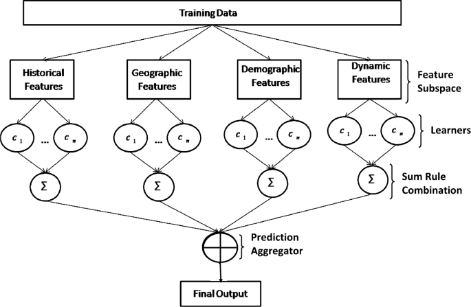
Ensemble model for crime event prediction
-
The third step ensembles the component classifiers for each training subset separately. We combine the output of the component classifiers for each subset. Among different types of combination technique, we use the sum rule in our ensemble model as it outperforms the other fixed rules [50]. Specially, the combination method applied in this work is
$$ O_{s}=\sum_{j\in C}O_{js}, $$(11)where C is set of classifiers and \(O_{js}\) is the outcome of classifier j on training subset s.
-
The fourth step aggregates the outcomes of each feature subsets for the final outcome. We train an SVM learning algorithm to aggregate the predictions made by each training subset.

6 Experiments
In this section, the experiment results are reported and discussed. The data used in the experiments is introduced in Sect. 3. The aim of the experiments is to examine the effectiveness of the dynamic features to crime event prediction at different settings.
6.1 Data preparation
First, we partition a day into 3 hours interval. Given a region, we predict whether it will be a hot spot in the next time interval for a particular type of crime (in other words, predict whether at least one crime event of a particular type will happen in this region in the next interval). Most of the existing works focused on comparatively long term crime prediction e.g. 1 day, 1 year. With the aim for short-term crime event prediction a day is divided into total eight intervals and each interval spans 3 hours. Crime prediction in finer temporal grain will help the police to design their patrol strategies dynamically and it will increase the probability to reduce crime rate more effectively. The shorter span of time interval, e.g., 1 hour, is better for short-term crime prediction. However, crime is a rare event and inter-sharing time of check-ins is high. Hence, we aggregate 3-hours interval data in our study.
As discussed in Sect. 5, it is hard to find many regions within a specified time interval where dynamic features exist and a particular type of crime event occurs. This makes it difficult to train a useful prediction model. So, the matrix factorization based method is applied to estimate the missing dynamic features as discussed in Sect. 5.1. In this experiment, the prediction models with dynamic features are trained after the estimation of missing dynamic features.
We partition the data in about 70% as the training set and the rest 30% as the test set for both cities, Brisbane and New York City. Particularly, in Brisbane, the data lies between 01/02/2013–30/06/2013 is considered as the training set and between 01/07/2013–16/09/2013 as the test set. In New York City, the training set involves the data between 03/03/2012–31/10/2012 and the data between 01/11/20112–15/02/2013 are test set.
Again, the occurrence of crime event is rare. So, most of the data are labeled with no-crime and few of the data are labeled with a particular type of crime event. This causes the data imbalance problem. To address this issue, we apply the under-sampling technique which drops some of the no-crime data at random to generate a balanced dataset. We train the prediction models using the balanced training set. The evaluation uses the original test set. As Brisbane is considered a relatively safe city, the balanced data of this city contain 30% crime data and 70% no-crime data. In New York City, the training data is balanced as 50% crime data and 50% no-crime data.
Most of the existing crime event prediction models used AUC, F1-score, Accuracy as their evaluation metrics [4, 13, 19]. Hence, In this paper we have chosen the Area Under Curve (AUC) under Receiver Operating Characteristic (ROC) curve, Accuracy, F1-score as the evaluation metrices.
6.2 Effectiveness of dynamic features
Five prediction models have been applied. They are the Random Forest (RF), Neural Network (NN), kernel Support Vector Machine (SVM), Logistic Regression Model (LR), and the introduced ensemble method (Ensemble). In particular, the Radial Basis Function (RBF) kernel is used in SVM. RBF is a real-valued function which calculates the Euclidean distance of the input variables from its origin [51]. We measure the performance of each model trained on combination of the historical, geographic and demographic features and then combining them with the dynamic features, for different types of crime event including Theft, Drug Offence, Assault, Fraud, Unlawful Entry and Traffic Related Offence during different time intervals.
6.2.1 Brisbane
The test results of AUC values with RF, NN, SVM, LR and Ensemble models are shown in Table 4. We observe the improvement of the AUC values after adding the dynamic features within different time intervals for different types of crime event. While the prediction performance varies based on the type of crime event and time interval for most of the prediction models, the RF shows the consistent improvement of AUC values after adding the dynamic features. In specific, with RF within different time intervals, the AUC values increase up to 4% after considering the dynamic features for Theft, 4% for Drug Offence, 16% for Assault, 2% for Fraud, and 6% for Unlawful Entry. No improvement has been observed for Traffic Related Offence. The test results verify that the dynamic features are significant to predict different types of crime event except for Traffic Related Offence. Interestingly, RF also possesses the best AUC values for all types of crime event within different time intervals. RF algorithm is consistent and adapts to sparsity. The convergence rate of the algorithm depends on only the strong features and hence, it is independent on the noise variables in the model [52]. For further evaluation, we report Accuracy% and F-1 score% with RF model in Table 5. We observe that the models with dynamic features yield better Accuracy% and F-1 score% than the models without dynamic features within different time intervals for different types of crime events.
6.2.2 New York City
The test results with RF, NN, SVM, LR and Ensemble models are shown in Table 6 for New York City. Like Brisbane, the improvement of the AUC values after adding the dynamic features is stable by using RF, compared to the others. It increases the AUC values up to 4% after considering the dynamic features for Theft, 4% for Drug Offence, 2% for Assault, 4% for Fraud, and 4% for Unlawful Entry. For Traffic Related Offence, the AUC value decreases or remains same after considering the dynamic features during most of the time intervals. Same as Brisbane, the experimental results in New York City prove the significance of dynamic features to predict different types of crime event except for Traffic Related Offence. The Ensemble model outperforms the others in terms of AUC values for all types of crime event within different time intervals. The Accuracy% and F-1 score% with RF model are reported in Table 7. Same as Brisbane, the models with dynamic features yield better Accuracy% and F-1 score% than the models without dynamic features within different time intervals for Theft, Drug Offence, Assault and Fraud. The performances slightly decrease within some time intervals for Unlawful Entry and Traffic Related Offence.
6.3 Significance test
In the above mentioned tests, we observe that the combination of dynamic features with static features can improve more or less the prediction performance for different types of crime event. To justify this improvement, we perform a statistical hypothesis test of RF model, more specifically, the paired t-test and report the results in this section. In this hypothesis test, the null hypothesis is \(\mathrm{AUC}_{\mathrm{wd}}\leq \mathrm{AUC}_{\mathrm{wod}}\), where \(\mathrm{AUC}_{\mathrm{wd}}\) is the AUC value with dynamic features and \(\mathrm{AUC}_{\mathrm{wod}}\) is the AUC value without dynamic features. The alternative hypothesis is \(\mathrm{AUC}_{\mathrm{wd}}>\mathrm{AUC}_{\mathrm{wod}}\). Here, we obtain a sample of \(\mathrm{AUC}_{\mathrm{wd}}\) and \(\mathrm{AUC}_{\mathrm{wod}}\) by applying 10-fold cross validation. The estimated p-value from the test can be observed in Table 8 for different types of crime event within different time intervals for two cities, Brisbane and New York City. The smaller p-value (less than 0.05) rejects the null hypothesis and accepts the alternative hypothesis. We observe small p-value for Theft within most of the time intervals in both cities. It proves that the dynamic features are significant in Theft prediction. Conversely, larger p-value for Traffic Related Offence at some time intervals justifies that dynamic features are less significant to predict this type of crime event. For the other types of crime event, the significance of the dynamic features depends on time interval and city. We can observe that the improvement after adding the dynamic features are statistically significant for more types of crime event within different time intervals in New York City than Brisbane. It proves that the availability of fineness human mobility data increases the significance of dynamic features in predicting different types of crime event.
6.4 Individual dynamic feature
For the different types of dynamic feature, the effectiveness in crime event prediction is not the same. We evaluate the importance of each individual dynamic feature to predict a crime event. In particular, we report the test result for Theft prediction. However, the same analysis can be applied to the other types of crime event.
The effectiveness of a particular type of dynamic feature is measured to predict the crime event using Random Forest algorithm. A particular dynamic feature is included into the baseline, consisting of no dynamic features, to measure its effectiveness in our experiments. The experimental results are shown in Table 9. The higher values of the AUC under ROC curve of these results show the extent to which the dynamic feature improves the prediction performance. While we observe a significant improvement in most of the cases in these results, the effectiveness of each dynamic feature varies with respect to time interval and city. In particular, Visitor Homogeneity is the most important dynamic feature for Brisbane (4.8% improvement in AUC) and New York City (1% improvement in AUC) within the interval [21–24) and [15–18), respectively. On the other hand, Region Popularity and Visitor Ratio are the most important features for New York City (1.2% improvement in AUC) within the interval [21–24) and Brisbane (3.2% improvement in AUC) within the interval [15–18), respectively. We also observe that Region Popularity and Visitor Count show a slightly decreased AUC values for Brisbane and New York City, respectively, within the interval [21–24), which indicates them as a noise in Theft prediction. The fact that different dynamic features may prove more or less significant across cities, types of crime event, and time intervals signifies that the problem of crime event prediction is not trivial.
6.5 Static vs. dynamic features
The effectiveness of all features (including static and dynamic) is investigated with LR for Theft prediction. To make it comparable, all features are normalized in between 0 and 1 [20]. The coefficient of each feature in the LR model indicates the importance of the corresponding feature. The most important 12 features (6 positives and 6 negatives) in two time intervals are shown in Table 10 for Brisbane and New York City. The positive coefficient means that the feature is positively correlated with the occurrence of crime events and the negative coefficient denotes the opposite. We observe that historical features have the strongest correlation with the occurrence of crime event. In Brisbane, we observe that the most positively correlated feature is 30-days crime density while the most negatively correlated feature is 7-days crime density for both intervals. In New York City, they are seasonal density and 30-days crime density respectively. It reveals an interesting pattern that Theft happens in the same region but less frequently. That is, it does not happen weekly but happen monthly in Brisbane and it follows a seasonal pattern in New York City.
For the dynamic features within the interval [15–18), Visitor Count has positive correlation with Theft whereas Region Popularity and Visitor Homogeneity are negatively correlated with Theft in Brisbane. It is interesting that the opposite happens within the interval [21–24). In New York City, Observation Frequency is positively correlated with Theft within the both time intervals. On the other hand, Visitor Ratio is negatively correlated with Theft within the interval [15–18), which is Visitor Entropy within the interval [21–24).
7 Conclusion
This work assists in solving the crime event prediction problem with its focus on exploring relevant dynamic features. Specifically, we propose to use the features extracted from human mobility to represent the dynamics of a region. Compared with previous studies on crime event prediction where relatively static features were the focus, this work was motivated by the research findings in Criminology which hold that many human-related factors such as social diversity and population distribution are relevant to an area’s safety. By capturing human mobility data through social media, it allows us to improve crime event prediction in finer spatiotemporal granularity.
In our approach, the sparsity of dynamic features has been addressed by using matrix factorization to estimate missing dynamic features. The effectiveness of the estimated dynamic features has been verified by correlation analysis and extensive tests in crime prediction cases. Data sparsity in fine spatio-temporal granularity is common in analysis of activity in urban spaces. Handling this issue successfully is essential no matter how advanced the analytic technologies which are applied. So, the contribution of this study is beyond the scope of the aimed research problems and will shed light on the field of spatiotemporal data analysis.
In future, we plan to extend our work in multiple ways. One of them is instead of verifying the model using data of same city only; we can use data from one city as training data and other one as test data. This could place the model verification in better way. However, the data distributions of different cities are vastly different. Hence, the problem needs to be formulated from transfer learning and domain adaptation point of view.
Abbreviations
- AUC:
-
Area Under Curve
- CARET:
-
Classification and Regression Tree
- CCDF:
-
Complementary Cumulative Distribution Function
- CCRBoost:
-
Cluster-Confidence-Rate-Boosting
- GAM:
-
General Additive Model
- GIS:
-
Geographic Information System
- GLM:
-
General Linear Regression Model
- KDE:
-
Kernel Density Estimation
- LBSN:
-
Location Based Social Network
- LDA:
-
Latent Dirichlet Allocation
- LDA:
-
Linear Discriminant Analysis
- LR:
-
Linear Regression
- NN:
-
Neural Network
- POI:
-
Point of Interest
- RBF:
-
Radial Basis Function
- RF:
-
Random Forest
- ROC:
-
Receiver Operating Characteristic
- SRL:
-
Semantic Role Labeling
- SVM:
-
Support Vector Machine
- 1NN:
-
One Nearest Neighbor
References
Yu C-H, Ward MW, Morabito M, Ding W (2011) Crime forecasting using data mining techniques. In: 2011 IEEE 11th international conference on data mining workshops, pp 779–786
Cohn EG (1990) Weather and crime. Br J Criminol 30(1):51–64
Zheng Y, Capra L, Wolfson O, Yang H (2014) Urban computing: concepts, methodologies, and applications. ACM Trans Intell Syst Technol 5(3):38
Gerber MS (2014) Predicting crime using Twitter and kernel density estimation. Decis Support Syst 61(1):115–125
Wang X, Gerber MS, Brown DE (2012) Automatic crime prediction using events extracted from Twitter posts. In: International conference on social computing, behavioral-cultural modeling, and prediction. Springer, Berlin, pp 231–238
Wang X, Brown DE, Gerber MS (2012) Spatio-temporal modeling of criminal incidents using geographic, demographic, and Twitter-derived information. In: Intelligence and security informatics (ISI), 2012 IEEE international conference on, pp 36–41. IEEE
Jacobs J (1961) The death and life of American cities
Ribeiro AIJT, Silva TH, Duarte-Figueiredo F, Loureiro AAFF (2014) Studying traffic conditions by analyzing Foursquare and Instagram data. In: Proceedings of the 11th ACM symposium on performance evaluation of wireless ad hoc, sensor, & ubiquitous networks. ACM, New York, pp 17–24
Silva TH, Vaz de Melo POS, Almeida JM, Salles J, Loureiro AaF (2013) A comparison of Foursquare and Instagram to the study of city dynamics and urban social behavior. In: Proceedings of the 2nd ACM SIGKDD international workshop on urban computing—UrbComp ’13, p 1
Ratcliffe J (2010) Crime mapping: spatial and temporal challenges. In: Handbook of quantitative criminology. Springer, Berlin, pp 5–24
Ratcliffe JH (2006) A temporal constraint theory to explain opportunity-based spatial offending patterns. J Res Crime Delinq 43(3):261–291
Perry WL (2013) Predictive policing: the role of crime forecasting in law enforcement operations. Rand Corporation
Yu CH, Ding W, Morabito M, Chen P (2016) Hierarchical spatio-temporal pattern discovery and predictive modeling. IEEE Trans Knowl Data Eng 28:979–993
Wang X, Brown DE (2011) The spatio-temporal generalized additive model for criminal incidents. In: Intelligence and security informatics (ISI), 2011 IEEE international conference on, pp 42–47. IEEE
Felson M, Clarke RV (1998) Opportunity makes the thief. Police research series, paper 98
Yu C-H, Ding W, Chen P, Morabito M (2014) Crime forecasting using spatio-temporal pattern with ensemble learning. In: Advances in knowledge discovery and data mining. Springer, Berlin, pp 174–185
Mohler GO, Short MB, Brantingham PJ, Schoenberg FP, Tita GE (2011) Self-exciting point process modeling of crime. J Am Stat Assoc 106(493):100–108
Cheetham R (2010) Hunchlab: spatial data mining for intelligence-driven policing. In: The annual meeting of the association of American geographers, pp 15–18
Bogomolov A, Lepri B, Staiano J, Oliver N, Pianesi F, Pentland A (2014) Once upon a crime: towards crime prediction from demographics and mobile data. In: Proceedings of the 16th international conference on multimodal interaction. ACM, New York, pp 427–434
Wang H, Kifer D, Graif C, Li Z (2016) Crime rate inference with big data. In: Proceedings of the 22nd ACM SIGKDD international conference on knowledge discovery and data mining. ACM, New York, pp 635–644
Wang H, Li Z (2017) Region representation learning via mobility flow. In: Proceedings of the 2017 ACM on conference on information and knowledge management. ACM, New York, pp 237–246
Zhao X, Tang J (2017) Modeling temporal-spatial correlations for crime prediction. In: Proceedings of the 2017 ACM on conference on information and knowledge management. ACM, New York, pp 497–506
Kadar C, Iria J, Cvijikj IP (2016) Exploring Foursquare-derived features for crime prediction in New York City. In: The 5th international workshop on urban computing (UrbComp 2016). ACM, New York
Kadar C, Brüngger RR, Pletikosa I (2017) Measuring ambient population from location-based social networks to describe urban crime. In: International conference on social informatics. Springer, Berlin, pp 521–535
Yang D, Zhang D, Qu B (2016) Participatory cultural mapping based on collective behavior data in location-based social networks. ACM Trans Intell Syst Technol 7(3):30
Yang D, Zhang D, Chen L, Qu B (2015) Nationtelescope: monitoring and visualizing large-scale collective behavior in lbsns. J Netw Comput Appl 55:170–180
Yang D, Zhang D, Zheng VW, Yu Z (2015) Modeling user activity preference by leveraging user spatial temporal characteristics in lbsns. IEEE Trans Syst Man Cybern Syst 45(1):129–142
Townsley M, Homel R, Chaseling J (2003) Infectious burglaries. A test of the near repeat hypothesis. Br J Criminol 43(3):615–633
Eck J, Chainey S, Cameron J, Wilson R (2005) Mapping crime: understanding hotspots
Nolan JJ (2004) Establishing the statistical relationship between population size and ucr crime rate: its impact and implications. Eur J Crime Crim Law Crim Justice 32(6):547–555
Chainey S, Ratcliffe J (2013) GIS and crime mapping. Wiley, New York
Michael RP, Zumpe D (1983) Sexual violence in the United States and the role of season. Am J Psychiatr 140(7):883–886
Poyner B, Webb B (1992) Reducing theft from shopping bags in city center markets. Situational crime prevention: successful case studies, pp 99–107
Sherman LW (1995) Hot spots of crime and criminal careers of places. Crime Place 4:35–52
Shannon CE (2001) A mathematical theory of communication. Mob Comput Commun Rev 5(1):3–55
Karamshuk D, Noulas A, Scellato S, Nicosia V, Mascolo C (2013) Geo-spotting: mining online location-based services for optimal retail store placement. In: Proceedings of the 19th ACM SIGKDD international conference on knowledge discovery and data mining. ACM, New York, pp 793–801
Hristova D, Williams MJ, Musolesi M, Panzarasa P, Mascolo C (2016) Measuring urban social diversity using interconnected geo-social networks. In: Proceedings of the 25th international conference on world wide web, pp 21–30. International World Wide Web Conferences Steering Committee
Cranshaw J, Toch E, Hong J, Kittur A, Sadeh N (2010) Bridging the gap between physical location and online social networks. In: Proceedings of the 12th ACM international conference on ubiquitous computing. ACM, New York, pp 119–128
De Nadai M, Staiano J, Larcher R, Sebe N, Quercia D, Lepri B (2016) The death and life of great Italian cities: a mobile phone data perspective. In: Proceedings of the 25th international conference on world wide web, pp 413–423. International World Wide Web Conferences Steering Committee
Quercia D, Saez D (2014) Mining urban deprivation from Foursquare: implicit crowdsourcing of city land use. IEEE Pervasive Comput 13(2):30–36
Venerandi A, Quattrone G, Capra L (2016) City form and well-being: what makes London neighborhoods good places to live? In: Proceedings of the 24th ACM SIGSPATIAL international conference on advances in geographic information systems. ACM, New York, p 70
Do TMT, Gatica-Perez D (2014) The places of our lives: visiting patterns and automatic labeling from longitudinal smartphone data. IEEE Trans Mob Comput 13(3):638–648
Koren Y, Bell R, Volinsky C (2009) Matrix factorization techniques for recommender systems. Computer 42(8):30–37
Cortes C, Vapnik V (1995) Support-vector networks. Mach Learn 20(3):273–297
Boser BE, Guyon IM, Vapnik VN (1992) A training algorithm for optimal margin classifiers. In: Proceedings of the fifth annual workshop on computational learning theory. ACM, New York, pp 144–152
Breiman L, Friedman J, Stone CJ, Olshen RA (1984) Classification and regression trees. CRC Press, Boca Raton
Fisher RA (1936) The use of multiple measurements in taxonomic problems. Ann. Eugen 7(2):179–188
Ho TK (1995) Random decision forests. In: Document analysis and recognition, 1995, proceedings of the third international conference on, vol 1, pp 278–282. IEEE
Liaw A, Wiener M (2002) Classification and regression by randomforest. R News 2(3):18–22
Kittler J (1998) Combining classifiers: a theoretical framework. Pattern Anal Appl 1(1):18–27
Buhmann MD (2003) Radial basis functions: theory and implementations, vol 12
Biau G (2012) Analysis of a random forests model. J Mach Learn Res 13:1063–1095
Acknowledgements
We thank all the CRUISE members for helpful discussion.
Availability of data and materials
Data and materials are available upon request.
Funding
Not applicable.
Author information
Authors and Affiliations
Contributions
SKR, KD and FS equally scoped the research. SKR formulated the initial idea, conducted the computational experiments and drafted the manuscript. KD and FS revised the problem formulation, guided the experiments and drafted the manuscript. All authors read, edited and approved the final manuscript.
Corresponding author
Ethics declarations
Competing interests
The authors declare that they have no competing interests.
Additional information
Publisher’s Note
Springer Nature remains neutral with regard to jurisdictional claims in published maps and institutional affiliations.
Rights and permissions
Open Access This article is distributed under the terms of the Creative Commons Attribution 4.0 International License (http://creativecommons.org/licenses/by/4.0/), which permits unrestricted use, distribution, and reproduction in any medium, provided you give appropriate credit to the original author(s) and the source, provide a link to the Creative Commons license, and indicate if changes were made.
About this article

Cite this article
Rumi, S.K., Deng, K. & Salim, F.D. Crime event prediction with dynamic features. EPJ Data Sci. 7, 43 (2018). https://doi.org/10.1140/epjds/s13688-018-0171-7
Received:
Accepted:
Published:
DOI: https://doi.org/10.1140/epjds/s13688-018-0171-7